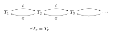
This book develops the surface-order and cyclic-time constructions of the supplied Emergent cyclic time manuscripts together with the subsequent projective-resolution, arithmetic and spectral work. The originals remain immutable. Their final unconditional GRH claims do not survive the identified arithmetic and operator-theoretic gaps. Here every construction has a specified category, coefficient field and determinant target. Established results, conditional implications, computed experiments and open comparisons play different roles.
The first two parts give the shared article constructions and their expanded proofs. The next part develops entire AR components, corrects the face-unfolding and Hom-control claims, and relates valid meshes to derived triangles and determinantal semi-invariants. The physics part retains the original topics while replacing invalid positivity, hardware and continuum inferences by proved finite statements or explicit research models. Computational chapters supply trained finite neural architectures, higher-genus dessins and a local interactive companion. The final comparison problem remains an independent arithmetic theorem, not a consequence of the pictures or learned parameters.
A reader may start with cellular dessins and the node, then projective resolutions, then the AR atlas. The more advanced arithmetic chapters use character sums and Fredholm determinants. The physics chapters can be read with finite-dimensional linear algebra and elementary quantum mechanics. Each computational claim has a script, seed and stated backend. The genus-two and genus-three sheet views are projections; the torus views are topological embeddings, not asserted uniformizing metrics.
The provenance manifest records the source hashes and chapter inventory. Its location is book/source-provenance.json. The review records state the audit coverage. The supplied 2053 file is byte-identical to the pinned source called COMPLETED in the source clone; the other supplied COMPLETED file is a shorter, different version. This naming discrepancy is retained in the provenance record. No filename certifies a theorem.
The companion is served on this machine at http://127.0.0.1:8765. It contains adjustable dessins, category-labelled AR diagrams, quantum carrier circuits, and saved training curves. The public repository and its project page provide the authoritative source and hosted companion. Selected lemmas are checked in Lean4; a full formalization of this entire book has not yet been completed.
We start with the surface-order constructions of Schreiber [1, 2], retaining the original sources unchanged. The generic-resolution source [3] is background, not a substitute for exactness of a particular complex. All primary algebra examples below come from explicit clean Belyi maps. Finite-dimensional objects occur as modules or specified quotient strata of those infinite algebras, not as replacements for them. The initial arithmetic target is a primitive nonprincipal Dirichlet -function. Finite-order Hecke characters, Dedekind zeta functions and general Artin representations require separate comparison theorems; Artin holomorphy is not assumed.
A clean dessin on a compact oriented surface is specified by a nonempty finite dart set , a fixed-point-free involution , and a permutation such that is transitive. Contract the white vertices of degree two. The resulting cellular graph has vertices the -orbits, edges the -orbits, and faces the -orbits, where
Write . Our quiver has vertices these edges and arrows . Paths are composed in travel order: traverses first. Set
Each vertex has two incoming and two outgoing arrows. Each arrow has precisely one permitted successor and one forbidden successor ; these are distinct because has no fixed points. The same holds for predecessors. This is the locally gentle condition. Every permitted cycle repeats indefinitely, so is infinite dimensional. We reserve “gentle” without qualification for the convention additionally imposing finite dimension.
Proposition 1.1 (The actual split order). For a permitted cycle of length , let be the hereditary cycle order in : diagonal and forward matrix entries are in , and entries crossing the chosen cycle cut are in . Then is the suborder of whose two diagonal constant terms labelled agree. With acting by , it is finite free of rank ; the conductor contains .
Proof. In a cycle order a path of length less than is the corresponding matrix unit, multiplied by exactly when it crosses the cut; another full turn multiplies it by . Thus completed paths in each permitted branch give all entries of . An arrow belongs to only that branch, whereas has diagonal entries at both occurrences . Hence the only condition on branchwise formal coefficients is the displayed equality of diagonal constants. This proves both injectivity and surjectivity of the path-normal-form identification. Multiplication respects it: switching branches across a paired edge is precisely a forbidden pair. The quotient is killed by , so the submodule has the same generic rank as . It is torsion free and finite over the DVR , hence free of that rank. The path and -adic topologies agree: , and if is the longest permitted cycle, any path of length at least is times a shorter nonempty path. Thus . This also justifies the completion used in the identification. □
The path-degree variable below is not : one full turn has path degree but -degree one. Formal, Laurent and operator-norm completions will likewise remain distinct.
Here are five explicit global inputs. Permutations list darts starting at zero; .
| Surface and Belyi map | |||
| , | |||
| , | |||
| , | |||
| , | |||
| , | |||
The first is the nodal interval: and . The second has , still infinite dimensional. The two theta dessins have the same two permitted three-cycles but different face cycles, respectively and . The elliptic square has one permitted and one forbidden four-cycle. For example has pole order two on the cubic ; has ramification above zero, above one since , and above infinity. The rational theta map has passport . These ramification computations, and the analogous direct zeros/poles in the other rows, verify cellular Belyi inputs rather than merely abstract quivers.
Use right modules , . Internal shift places its old generator in degree . Let be the indexing words of length from with every adjacent pair forbidden, including for . Such a word is usually zero in ; it still labels a summand.
Theorem 2.1 (Exact resolutions). There is a minimal graded projective resolution, with and for ,
The augmentation is the quotient. For the completed order the identical finite-rank projective terms and formal-series maps resolve the residue simple. Ext and Tor against residue simples count forbidden words with the prescribed endpoints. In the graded case Ext has matching internal shift .
Proof. The maps are right linear and degree zero. Adjacent differentials multiply by a forbidden pair. The augmentation kernel is the direct sum of over initial arrows. For any arrow , multiplication kills exactly the permitted paths beginning with its forbidden successor . All other basis paths survive to distinct basis paths. Thus its kernel is . For a fixed prefix, different last arrows have disjoint surviving supports; there is no cancellation between summands. This proves exactness inductively. For formal series the same assertion holds coefficient by coefficient and identifies the entire closed kernel, not just its dense polynomial subspace. Terms are idempotent projectives and all entries are arrows. Consequently applying Hom or tensor with a residue simple kills every differential, proving minimality and the Ext/Tor count. In minimality is graded; it does not require that be its ordinary Jacobson radical. □
The two arms never terminate in this closed class. Their labelled patterns follow -cycles. An ungraded positive syzygy tail can have a shorter period by permutation of summands: the nodal interval has labelled period two but unordered tail period one; the elliptic theta has labelled period six and unordered tail period three. A simple need not be isomorphic to a positive syzygy; for the node it is -torsion, whereas the positive syzygies are lattices.
Let and . Degreewise Euler characteristic of the resolution gives : every coefficient is finite, because a summand in homological degree starts in internal degree . Constant terms are , so the inverse is two-sided. Already signed must not be evaluated at again.
Proposition 2.2 (Dual dessin and cycle determinant). The complementary-relation algebra is another closed dessin algebra, with , , permitted successor , and forbidden successor . It exchanges graph vertices and faces and preserves genus. Its Cartan matrix satisfies , with the opposite convention if required for Yoneda composition. For independent commuting arrow weights ,
Proof. , so the claimed relations and face data follow directly; the connectedness group is unchanged. To prove the determinant, put when , and when , zero otherwise. On arrow states let for permitted adjacency and for forbidden adjacency. Then and the path sum is . Sylvester’s identity gives . Each transition is a weighted permutation, whose cycle determinant is respectively and . Everything holds in formal power series, hence as rational functions. This supplies a direct proof of the Bessenrodt–Holm formula in the closed dessin class [4]. □
The five univariate determinants are, in the order above,
The last cancellation does not imply finite global dimension: its forbidden resolution is infinite. These rational functions have cycle poles/zeros, not arithmetic prime Euler factors.
For clarity, a complex is a sequence with , its homotopy category identifies maps differing by , and inverts maps inducing cohomology isomorphisms. A perfect complex is represented by a bounded complex of finite projectives. Our infinite simple resolutions compute derived Hom and tensor but are generally not perfect. The two-term presentation is perfect even if its kernel is nonzero. Quadratic linearity is a Koszul statement; it is not by itself an equivalence between all completed derived categories. Likewise a finite-dimensional gentle graded-curve theorem [6] cannot simply be transferred to these closed infinite orders. Here the surface walks explicitly compute the resolution endpoints: turns round a graph vertex and follows a face. For longer string objects all maps can be computed from the occurrence matrices; a universal geodesic-intersection classification for this completed category remains a separate theorem.
The two filtration parameters below are not dessin arrows. Let for a field , and let , , where ,
The positive outer exponents make finite length. Write for a free generator born in bidegree .
Proposition 2.3 (Adjacent syzygies). A minimal bigraded free resolution of is
where and . Deleting row from gives determinant . The Hilbert series numerator is .
Proof. Each column maps to zero. In a relation , all terms except the last contain . Coprimality with implies . Subtract from the coefficient vector; its last component vanishes. Factor from the remaining generators. They form a smaller staircase with the same strict inequalities, ending in a pure -power. Induction expresses the remaining relation in the preceding adjacent columns. The base of one generator has no relations, since is a domain. Hence . If , its first row gives ; successive rows then force all . This proves injectivity. Every differential entry has positive degree, so reduction modulo kills the differentials and the resolution is minimal. In the row-deleted matrix the unique nonzero permutation term uses the negative entries before row and the positive entries after it. Their exponents telescope to , respectively, and the sign is . Finally take the degreewise Euler characteristic; the free summands have Hilbert denominator . □
For the underlying sequence is also kernel checked in Lean 4 over the actual ring . The verification proves the kernel/image equalities, the stated ideal image, surjective quotient augmentation, projective free terms, and vanishing of both induced Hom differentials to the constant-coefficient residue field. It uses regular multiplication on the free modules, distinct from the residue action on . General staircases, graded minimality and the surface-order coefficient cone remain separately scoped prose arguments.
At grade , has dimension one exactly when no generator degree is componentwise at most . Its comparable-grade map has rank one exactly when both endpoint grades satisfy this condition. A CW realization takes one loop and attaches a disk once along it at each generator degree. The active indices form an interval: the inequality selects a final interval, the inequality an initial interval. With active disks, the cellular map has every entry one. Thus and , the latter counting active adjacent syzygies. This auxiliary CW complex is not the dessin surface.
For the actual nodal order put and . The basis of satisfies , , . Tensoring the resolution above with gives, over , free ranks . Indeed the scalar resolution stays exact after tensoring over the field; its degree-zero module is free over on the standard monomials. Multiplication by is injective there and on all free terms, so the long exact homology sequence of its mapping cone gives positive-degree homology zero and degree-zero module . In contrast, as an -module this object has ranks in its minimal resolution. Neither finite-length nor these parameter rings replace the infinite parent dessin algebra or its lattice category.
Proposition 2.4 (One common channel). Let be a positive trace-preserving linear map between finite complex matrix algebras. For density matrices , their trace distance satisfies . For finitely many labelled states, keep fixed vertex birth grades . At include vertices with and edges with distance at most , and take the flag complex. Then gives an identity-on-labels inclusion from the input to the output bifiltration, natural in .
Proof. Write the Hermitian difference as with . Positivity, the trace norm triangle inequality and trace preservation give . Thus every input edge is an output edge; the fixed births preserve vertices, and all cliques are preserved. Increasing either parameter preserves the simplices, and every map is the same label inclusion, so the squares commute. Complete positivity is sufficient but is not needed for this norm argument. □
For a finite inclusion , work over a field and embed a basis of source one-cycles into the target edge space. If is the matrix of target two-boundaries, the induced rank is
Its image is ; source boundaries already map into target boundaries. This proves the formula, including empty complexes. Computing a flag two-skeleton suffices for , but does not compute the full flag complex’s . Integer ceilings of scaled exact distances preserve the inclusion. For numerical distances, frozen integer labels define an exact combinatorial diagram only after their inequality is checked; this is not an interval certificate of the underlying quantum distances. None of these finite ranks identifies a completed arithmetic determinant or proves GRH.
Use cohomological degrees and an uncurved differential of degree . An odd element with contracts the underlying -complex of every unital left DG module: satisfies by the graded Leibniz rule. Thus this example has zero cohomology, contrary to the original ground-field-resolution claim. An isomorphism on alone is also insufficient for a DG quasi-isomorphism; all degrees must be checked.
Proposition 2.5 (Nodal Koszul model). Let be a field, and and , with , , and . The augmentation , , is a DG-algebra quasi-isomorphism onto the actual infinite nodal dessin algebra. Branch rescaling , , for lifts to a DG automorphism.
Proof. Multiplication is . The differential kills degree zero and sends to . Its square is zero. For two odd inputs the Leibniz right side is ; the other homogeneous cases follow by -linearity. Multiplication by is injective in the polynomial domain. Hence , , and all other groups vanish. The augmentation preserves products and kills boundaries. Rescaling fixes , so its coefficientwise extension commutes with and has inverse obtained by replacing with . This is a one-relation Koszul construction [78, 79]. □
Replacing by gives the completed order: setting each variable separately to zero maps onto the branch pullback, and the kernel consists precisely of mixed monomials, hence equals . Rescaling is generally semilinear over the coefficient ring, rather than linear over the fixed diagonal DVR , . It preserves that DVR as a subring exactly when , and fixes it pointwise exactly when . No Hilbert norm or arithmetic spectrum follows.
The corresponding Lean file checks the actual exterior-line algebra, differential, sign-Leibniz, homotopy and polynomial ambient-resolution identities. Full graded/category/completion objects remain separately scoped. The two theta dessins likewise require endpoint-sensitive Ext: self is zero in both; for the elliptic theta self has dimension two, while for the spherical theta positive even self Ext has dimension two. Outdegree alone does not count self extensions. Minimal models use additional graded data [77, §3.3]; is not automatically a physical curvature.
Assume algebraically closed of characteristic zero for invariant-ring statements. A finite-dimensional representation of the infinite has spaces , arrow matrices satisfying the monomial relations, and base-change group . With column vectors, . Let , , and be a finite path-matrix map. When , define
It is intrinsically a determinant-line section; chosen bases give this scalar.
Proposition 3.1 (Weights and exact homological scope). . Restricted determinants of this form span all semi-invariants on a closed -stable relation or nilpotence locus. Set . On the square locus,
If is injective, and higher Ext vanish. Without injectivity neither that cokernel equality nor higher vanishing follows.
Proof. Naturality gives , where repeats the relevant . Take determinants. The contragredient coordinate-ring action has the inverse character. Schofield–van den Bergh’s spanning theorem allows oriented cycles [36, Theorem2.3]. Exactness of invariants for reductive in characteristic zero lifts a fixed-weight function from any closed stable locus to the ambient representation space; restrict the spanning determinants. Injectivity of the path map need not survive that restriction. Finally . Writing , the exact sequence with projective expresses as ; the epimorphism embeds this quotient in . A square finite matrix with zero kernel has zero cokernel. If is injective it is the actual length-one resolution, giving the stronger assertion. □
For the node, , , give but . For the elliptic square name arrows so that , , permitted cycle and forbidden cycle . With and , , its Hom matrix is , yet the subsequent forbidden resolution gives . Thus nonvanishing is not all-degree derived orthogonality.
Proposition 3.2 (What completion does to invariants). A continuous -dimensional representation of kills . On the reduced nilpotent representation variety of fixed dimension vector every invariant regular function is constant. Nonzero-weight semi-invariants need not be constant.
Proof. Continuity with discrete finite-dimensional target kills some ; its Loewy filtration has at most nonzero strict steps. Choose vertexwise complements to this filtration. An arrow sends a layer into layers . Scaling layer by conjugates each component by . At the representation tends to the zero-arrow representation. Every invariant therefore has the same value at all points; reducedness and the Nullstellensatz give the ring assertion. In the square example the scalar varies on a nilpotent locus and has weight , so semi-invariants survive. Formal entries in a projective map are evaluated on this locus by truncating modulo , a legitimate finite polynomial operation. □
On the node, is regular and is free of rank two over . The polynomial presentation for is injective and its determinant on is , the characteristic polynomial of up to the sign . But is a unit in , with its geometric-series inverse, so those modules do not extend continuously to the completion. An -free lattice and its -nilpotent quotients are different categories. On a lattice a separately specified endomorphism has a meaningful relative characteristic polynomial over ; the scalar base action alone does not create Frobenius.
For a nonempty partition , choose a numbering of its boxes. On let , the unnormalized row sum followed by the signed column sum. The classical identity , where is the hook product, makes an idempotent in characteristic zero. Its image is , one Schur copy, rather than the whole symmetric-group isotypic component [31, 32]. Its character is , computed by semistandard tableaux (weak rows, strict columns), and
Since commutes with the place permutations, it induces and respects composition and zero maps. Applying this at every vertex and arrow therefore gives a genuine representation of the monomial dessin algebra: for a forbidden pair. The empty partition does not have this property: it sends zero arrow maps to the identity of .
The Littlewood–Richardson rule gives natural intertwiners
Here counts semistandard tableaux of skew shape and content whose row-reading word is Yamanouchi. Naturality makes the same decompositions intertwine all the arrows. The tensor operation is vertexwise with synchronous arrow maps, not and not a Hopf-algebra tensor structure. There is no automatic tensor unit preserving these zero relations. These functors are not additive or exact; they cannot simply be applied degreewise to a projective resolution. They also need not preserve the fixed -action on lattices.
In the elliptic theta set one of the two permitted three-cycle branches to zero. The other has arbitrary maps , , , with all spaces of dimension . This is a closed representation stratum of our infinite dessin algebra. Put .
Theorem 3.3 (Cyclic invariants and a local positive kernel). The invariant ring on this stratum is , where are characteristic coefficients. Its total-arrow-degree Hilbert series is . Common multidegree has basis , , ; other multidegrees have no invariants. Products obey the Littlewood–Richardson rule. Over , if and and , the kernel
is absolutely convergent and positive semidefinite.
Proof. Cycle-trace generation for quivers, including relation quotients, is the Le Bruyn–Procesi theorem [29, 30]. Every cycle here is a power of the full three-cycle, up to cyclic rotation. In characteristic zero Newton identities give the generators . They are algebraically independent: take and arbitrary . Scalar changes at the three vertices force equal arrow multidegrees. Restriction to that same section identifies degree with degree- symmetric polynomials in eigenvalues, whose Schur basis and product rule give the assertion. For the kernel use the ordinary Cauchy identity, first as a formal identity in eigenvalues. On Schur modules the operator norm of is at most , so its trace is bounded by . The dimension Cauchy identity bounds the absolute series by . Each summand is a rank-one Gram kernel, proving positivity by absolute summation. □
The term for the empty partition is a constant scalar feature, not an allowed module-valued tensor unit. In dimension two,
More generally and its reciprocal is . These are actual determinant/Schur connections, not identifications with an arithmetic -function. On continuous finite-length -modules the monodromy is nilpotent and all positive-degree characters vanish. The displayed Cauchy positivity is local representation-theoretic positivity, not the global Weil form.
For the interval dessin let , in , , . A lattice is a finitely generated -module free over .
Theorem 4.1 (The nodal lattice calculation). Every lattice is . The almost-split sequences in this lattice category are
In particular , . Multiplication by between two copies of either row, followed by reduction modulo , gives an actual nonzero exact three-by-three diagram.
Proof. Normalize inside its total quotient module: , . The conductor gives . Both branch projections of are onto. Intersect with the two factors; its remaining quotient identifies their two residual quotients. Separate bases for these pure factors and the common quotient put into pure first lines, pure second lines and diagonal pairs. Lift branch bases over the DVRs. These are respectively the summands . Their endomorphism rings are local.
Exactness of the first sequence is . It does not split: a map lands in , and its composite with is a nonunit in . Every map factors through this epimorphism, , and every nonunit endomorphism of is divisible by and factors through . Classification handles all finite sums; a unit component would be a retraction. This is right almost splitness. The dual argument for nonsections out of proves left almost splitness. Endomorphisms fixing either structure map have constant term one, hence are units, proving minimality. Swap for the other sequence. Finally all three terms are -free. Multiplication by is injective and reduction preserves exactness, proving the diagram assertion. □
The lattice AR quiver has arrows and ; the mesh composites are zero. Its projective vertex is not the endpoint of another nonsplit AR sequence. AR meshes do not mean that all rows and columns of any drawn grid are short exact.
For a second, explicit family fix and the rational Belyi map
where are Chebyshev polynomials. It has passport . Its contracted dual graph is a path, identifying its genus-zero dessin. The associated infinite algebra has vertices , endpoint loops , opposite arrows , , and precisely the relations . Its single permitted cycle is ; the order rank is .
Retain one arrow at each edge in an orientation , and kill its opposite. The quotient is exactly the string algebra of Huang–Lin–Su [46]; the killed-arrow ideal contains , so it is also an actual quotient of . Inflation identifies its module category with the full abelian quotient-annihilator subcategory of -modules. This is generally not extension closed in the whole order category. The imported AR property is intrinsic to , not automatically an ambient lattice or finite-length AR property. The extended edition gives nine explicit string modules, all twelve maps and the four exact meshes from the supplied diamond resource, now situated in this actual dessin quotient.
The other supplied resources also have a precise home. For the interval order the subcategory annihilated by is , . This is a domestic string quotient, not itself a gentle algebra. Inflation is full and preserves purity, and is a closed subspace of . Ringel’s infinite-word/pure-injective program and its proof by Puninski–Prest apply there [43, 44]; the isolated band gives Krull–Gabriel and relative Cantor–Bendixson dimension two by [45, Theorem10.19]. This is not an ambient rank calculation for all -modules. The parameter in survives even though all cycle traces vanish; the pp condition detects it. These modules are -torsion and are not nonzero order lattices. Infinite-string and locally finite AR theorems must retain their distinct finiteness hypotheses; a surviving permitted cycle has infinitely many paths at a vertex.
Crawley–Boevey’s theorem [38, Theorems1.1–1.4] applies directly to the infinite polynomial dessin algebra: its finitely controlled modules decompose into strings and finite-dimensional bands; its pointwise artinian modules additionally allow primitive injective bands. For our finite quiver, these conditions mean finitely generated and artinian respectively. The words may be infinite, but their modules have algebraic direct-sum bases. This is not a classification of every module or of arbitrary formal completions.
In fact no nonzero completed-order lattice, restricted to , meets either finiteness condition. The polynomial is finite over : remove full turns from sufficiently long paths as in Proposition 1.1. If an -free lattice were finitely generated over , it would be finite torsion free, hence free, over the PID . Multiplication by would then fail to be onto, whereas it is a unit over . Also excludes artinianity. For a concrete indecomposable outside the ordinary string/band list take with : its endomorphisms are multiplication by formal series, so its endomorphism ring is local. Its is injective and nonsurjective, while is invertible; these properties exclude every pure- ordinary string or band. The extended edition gives the full word argument.
The Fukaya connection requires equally precise categories. Lekili–Polishchuk explicitly allow infinite-dimensional locally gentle algebras, but their equivalence is for perfect dg modules of a homologically smooth algebra, with specified grading, line field and stops [66, Definition3.1.1, Lemma3.1.3, Theorem3.2.2]. Every nonempty closed dessin here has both permitted and forbidden cycles, so its polynomial algebra is neither proper nor smooth by their criterion. This does not exclude appropriate singular or completed variants; it prevents a direct use of that particular theorem. Infinite word, graded curve and geodesic are not interchangeable without a surface realization and boundary/grading data.
There is a genuine positive example inside our setting: the polynomial interval quotient is still infinite dimensional, is smooth, and has no forbidden cycle. Its perfect category has the partially wrapped annulus model with one stop total. In degree zero . Inflation of this quotient is fully faithful on ordinary modules, but not on derived categories: , whereas . The former follows from the alternating resolution. Thus this quotient bridge does not identify the whole closed dessin’s perfect category with the annulus category.
Finally, Leavitt path algebras can fail invariant basis number, but need not. The permitted-state Laurent algebras here have finite-dimensional matrix quotients, and therefore invariant basis number. The polynomial and completed dessin algebras have their vertex-simple quotients, giving the same conclusion. The complex Leavitt algebra of below is a dense *-subalgebra of its graph C*-algebra, on that specified graph; it is not the original gentle algebra with ordinary CK1 imposed.
Work now over . Ordinary Leavitt and graph C* constructions [47, 48] cannot simply impose our original forbidden products: if and CK1 says , then . Every arrow is a forbidden successor, hence every arrow and then every vertex is zero. CK2 is not needed. The ordinary graph-Toeplitz CK1 setting has the same collapse.
The valid permitted-arrow-state graph instead consists of the disjoint directed -cycles. Its Leavitt algebra is , and its graph C* algebra is . These forget the -gluing; both theta dessins give the same answer. They are not the completed original order. Nor is the ordinary Toeplitz algebra of a cycle of length equal to : their ranks are and one respectively [50].
Let for all permitted finite paths, including vacua . Define when the prefix is permitted and composable, and zero otherwise. Let project onto paths starting at , and onto the vacuum. Then
These follow on basis vectors. The different initial projection avoids CK1 collapse. Write , a constrained-path Fock C* algebra in the monomial/subproduct setting [51, 52]. The polynomial acts faithfully: applying a finite path sum to the sum of vacua recovers its coefficients. This representation need not extend to all formal series: along a cycle would send its vacuum to a nonsquare-summable sum.
Theorem 5.1 (Compact extension and incidence index). Let be the terminal-path sector. There is an exact sequence
With , its boundary map is , minus the unsigned incidence map of the cellular graph. Thus, for its edges,
Proof. All prefixes preserve the terminal sectors. For paths ending at , . Therefore the vacuum ideal is exactly the displayed sum of compacts: it contains these matrix units and that sum is itself an ideal. In the quotient, has initial projection and range , a graph CK family for the permitted-state cycles. The have infinite rank and nonzero quotient images; the length gauge action descends. Gauge-invariant uniqueness [48, Theorem2.1] identifies the quotient as claimed.
For a cycle based at arrow , lift its corner unitary by . Then and projects onto the first paths starting with . Their terminal vertices count exactly its incident darts, including twice for a loop. This proves the index formula. The six-term exact sequence gives and . The free last term splits abstractly. Spanning-tree integer elimination gives Smith entries repeated times and one zero in the bipartite case; an odd cycle instead adds the entry two. This proves the groups. □
The nodal interval has , ; the single-loop sphere has , zero. Both theta dessins have , . Coarse -theory does not recover genus or the arithmetic factors.
The Fock algebra itself has a graph presentation, on a different graph from the original gentle quiver. Let have vertices for and sinks for , and edges
Proposition 5.2. , by , , and . The integer graph relation at is . Eliminating these relations recovers and .
Proof. The two edges at have orthogonal initial pieces and orthogonal ranges summing to , by the Fock initial-projection identity. All vertex projections are nonzero. The length gauge acts with degree one on both edge families, so gauge-invariant uniqueness applies. They generate since and . In the integer matrix a kernel coefficient is constant around each permitted cycle; its sink equations are exactly . In the cokernel, eliminate all but one state per cycle; its remaining relation is the sum of its incident sink generators. The remaining cycle generators are free, proving the stated groups. □
For the nodal interval, has two loop vertices, each with an exit to the common vacuum sink. Chirvasitu–Hajac–Tobolski’s actual pullback theorem [65, Theorem3.4] gives
where has the same three vertices and countably many arrows from each loop vertex to the sink, with no loops. The arrow numbered maps to loop followed by exit. This algebra is AF, with , . The extended edition verifies every hypothesis. The theorem does not turn arbitrary cycle-vertex identifications into pullbacks: its first graph is acyclic and its path functor must cover all pointed paths. Its sink-extension Theorem4.3 has further injection and path-coverage requirements.
The formal order’s residue gluing cannot be copied by taking diagonals of arbitrary full matrices: . For there is no nonzero *-homomorphism from to a commutative C*-algebra, as restriction to its constant matrix units shows. Restrict the distinguished fiber first. Define
where the first map evaluates diagonal entries at one and the second repeats at the two darts paired by .
Theorem 5.3 (A faithful polynomial pullback model). There is a split exact sequence
so and . The polynomial dessin algebra embeds faithfully and generates this C*-algebra with its adjoints. This embedding does not extend to a unital algebra map from all of .
Proof. The section consists of the constant paired diagonal projections. The kernel is the displayed vanishing fiber, a sum of matrix suspensions, giving the groups by split exactness and suspension. For an explicit embedding set , choose one cut arrow per permitted cycle, and send to in its branch, where at the cut and zero otherwise. Send to the constant paired diagonal projection. Every forbidden product is zero. A full cycle at maps to , . This scalar function is injective on the circle: away from its unique zero at one its argument recovers . Continuous functional calculus therefore supplies every with . Multiplying by path images and approximating division away from one supplies every vanishing off-diagonal entry. Together with the constant paired diagonals these generate . Path normal forms in a fixed entry are a nonzero prefactor times a polynomial in ; its infinite range proves independence. Evaluation at one first separates the zero-length coefficients. Finally for , is a unit in the formal order, but its proposed image is singular at . A unital map preserves units, proving nonextension. □
This is the C* algebra generated by a faithful polynomial representation and its adjoints, distinct from the completed order and from . The norm closure of the polynomial image alone need not contain those adjoints. Their groups already differ. The pairing belongs to the labelled presentation; an unmarked isomorphism class need not recover the ribbon ordering. No arithmetic descent, Frobenius action or completed- positive determinant is inferred from this additional valid gluing model.
Proposition 5.4 (The degree spectral triple). Define on . With the polynomial creation/annihilation *-algebra this is an ungraded spectral triple, -summable exactly for . With zero on the kernel,
for and in the last two formulas, where is an externally chosen Dirichlet character.
Proof. There are vacua and paths of every positive length: each starting arrow has a unique continuation. The real diagonal operator is self-adjoint on the stated maximal domain; finite supports are a core and its resolvent is compact. Prefixes preserve the domain and , , so polynomial commutators are bounded. The trace formulas and summability reduce to the corresponding scalar series. The character multiplier is bounded; membership in is not asserted. □
Length parity anticommutes with the creators but commutes with , so it is not an even-spectral-triple grading. The ordinary odd Fredholm class of this positive is trivial: is compact. The spectrum depends only on ; zeros of the scalar zeta trace are not eigenvalues of .
The compact ideal gives a precise home for an arithmetic determinant, with no claim that the arithmetic is derived from the dessin. Fix one terminal sector. Its two paths of each length give orthonormal vectors and an isometry .
For a nonprincipal character put , , and, on , set
Here . For , and the pairing is complex linear, with no conjugation of . Define
Indeed dyadic blocks give , and on a compact set , , the squared tail is bounded by . Thus the rank-one family is trace-norm holomorphic. Its determinant is , equal by Abel summation to . Replacing by and adding to the functional gives exactly every raw partial sum , with compact-uniform trace-norm convergence; . For primitive , completion replaces the functional by , with the standard nonzero gamma factor , rather than multiplying the whole old functional. The extended edition supplies the quantitative estimates.
This inserts a scalar encoding into one actual dessin compact ideal; it is not known to be -linear, a derived chain map or Frobenius compatible. A common fixed positive metric cannot make this same fixed-range family symmetric for all critical heights: symmetry forces its functionals to be proportional, whereas the coefficient ratio at heights is asymptotic to , with two opposite subsequential limits. Different positive realizations remain possible.
Proposition 6.1 (Complex dessin data do not determine arithmetic descent). The rational Belyi pairs , , for , are isomorphic over but have distinct Frobenius polynomials at the good prime seven: and .
Proof. Choose , . The projective isomorphism from to preserves the Belyi map. The degree-six clean passports are the elliptic theta passport already computed. Directly counting for gives respectively and . Including infinity yields four and seven points, hence . Both discriminants are nonzero modulo seven. □
Any invariant of the complex dessin or its undecorated order/Fock algebra alone is the same for these two inputs, so cannot recover both factors without descent data. This does not obstruct a theory including a specified rational model and compatible Galois action. Elliptic has weight one and unshifted center , unlike Dirichlet center ; the example is not a counterexample to GRH.
The preceding twists can be distinguished constructively once their finite-field descent data are retained. This closes the elementary local-factor computation, not the global positive-determinant problem. Let , and . Put and . For , fix a nontrivial cubic character and the quadratic character , both extended by zero at zero. Define
Theorem 6.2 (Uniform local factor). For every such prime power and nonzero ,
If , instead . The split-case values lie in , .
Proof. Cube fibers have size , including at zero; the first term is the literal constant one, not the zero-extended trivial character. Counting square fibers gives . Grouping by removes the constant term since . Substitution gives ; the other term is its conjugate. This proves the signed trace formula.
For a nontrivial additive character , write . Character orthogonality gives for nontrivial : substitute in its squared norm; the inner sum over is at and otherwise. Grouping by gives , the zero-sum fiber vanishing since is nontrivial. The three Gauss norms yield . Neither purity nor RH was assumed. The remaining signs and character values have modulus one. For cubing is bijective, so the quadratic-character sum is zero. Finally all split-case summands are signs times cube roots of unity. These are the classical Gauss–Jacobi methods [68, pp.499–502], with our normalization proved explicitly. □
At , choose . Then , , and , giving the two factors already counted. At , gives but ; this detects the essential sign hidden by the first example.
Assume in this cellular construction. The elliptic theta dessin has cellular chains , , . Orient the three edges from to ; then and . Thus is the sum-zero plane, with basis . Rotation acts there by
is the actual Euclidean edge Gram matrix in this basis. The deck involution acts as . Consequently the six-element deck group acts on this homology and permutes the original quiver and its entire projective resolution.
Write . Its multiplication action on this actual cellular plane is
This constructs the local matrix from finite-field character sums and the dessin’s deck action, rather than fitting its trace. Positivity follows from . The normalized matrix is -unitary, not asserted self-adjoint. The extended edition supplies a rational cellular chain lift, its exact determinant cancellation, and Kummer descent compatibility on homology. Its odd-over-even determinant ratio is the classical finite-field curve zeta function
Identification with the geometric -adic Frobenius polynomial uses the standard elliptic trace and determinant theorem; a canonical integral comparison or an order-derived Frobenius functor has not been constructed here.
There is also a precise obstruction to extending this same real two-dimensional carrier to . Frobenius then conjugates the cubic deck action. The relation forces , whose determinant is , contradicting the required positive determinant . This excludes that real carrier with its fixed deck action, not complex or enlarged Hilbert–Pólya constructions. The extended edition gives a compatible complex local replacement.
For the following insertion test use the characteristic-zero theta order over , with residue simple . The limitation is concrete. The deck action has finite order and cannot alone supply the norm- Jacobi coefficient. Inserting into gives an actual residue-module endomorphism with determinant , but that simple is not perfect over the order and choosing it breaks full deck symmetry. Inserting the same matrix -linearly into the regular projective instead gives the -determinant , or on . Taking a root is not an established determinant-line comparison; a deck-semilinear lift is a different map. These surviving multiplicity/equivariance obligations prevent promoting the local computation to the required arithmetic order functor.
For the global comparison fix a nonzero rational and use its good reductions. The finite-field curve zeta has center after . The global elliptic -function over has unshifted center one, whereas Dirichlet -functions have center . Local weight-one purity does not determine either global zero set. The elementary local bound proves absolute convergence of the elliptic Euler product on ; the new local identities give no determinant-preserving continuation with the desired global positive spectrum.
The preceding tensor test has a stronger replacement. Keep the characteristic-zero completed elliptic theta order over , and write . All determinants in the next theorem are ordinary underlying- determinants; they are not reduced norms.
Theorem 6.3 (Projective determinant multiplicity). Let be any finitely generated projective right -module and . Then . Let be the induced maps on its three top multiplicity spaces. Then
For any bounded complex of these projectives and any -linear chain endomorphism, its alternating determinant ratio specializes to a sixth power in . Generically, the ordinary ratio is a cube in .
Proof. The arrow ideal is the Jacobson radical: its elements admit geometric-series inverses after subtracting from one, and the quotient is . A projective’s top lifts to a map from the displayed sum; Nakayama gives surjectivity, projectivity splits it, and another application of Nakayama kills the kernel.
Put . Each has path layers of dimensions : the identity, two length-one paths, two length-two paths, and one length-three path. The two full cycles based at add to , so become negatives; all length-four paths vanish. A positive-length entry of a projective homomorphism strictly raises path length. Consequently the associated graded map has six copies of , giving the formula by triangular block determinants. Base change of determinants justifies specialization. Multiplicativity along filtrations is ordinary linear algebra, consistent with [69, Tags0FJ9,0GSX]; no purity assumption enters.
Each term’s determinant has constant term one in , so every denominator has nonzero specialization. Taking the finite alternating product therefore preserves the sixth power, even after cancellation. Finally ; a projective’s branch modules are sums of three-dimensional simples. A commuting endomorphism acts on each multiplicity space, repeating every factor three times. This proves the generic assertion. □
Thus no such ordinary perfect-complex ratio can equal the constant-in- quadratic , or the full local curve zeta . For , the valuation at infinity is , not a multiple of six. For the zeta ratio, by the local bound , so its pole at is simple. This also covers square prime powers where the numerator may have a double root. It is an obstruction for the specified ordinary determinant and linear category, not all spectral or determinant theories.
There is nevertheless a genuine integral functor removing this multiplicity. Choose a permitted branch and its cycle cut. Its projection makes the column lattice a left -module. Define
Bounded projectives compute this derived tensor functor; flatness of on all modules is unnecessary. Since , its determinant on with external action is exactly , whereas on the regular module it is . This is a defined change of determinant functor, not an arbitrary polynomial root. It does not construct the arithmetic action independently: the already computed is still the input.
The price of this repair is precise. Branch swap exchanges and ; pairing them yields on that basic-projective input. The chosen branch determinant cannot intertwine on all endomorphisms: the corner unit acting on , with a plus full cycle, acts on its determinant by , whereas its -image acts by one. Also no rank-one-per-vertex column lattice supported on one branch admits an -linear lift of the rotation fixing . Its three nonzero arrow scalars have nonnegative -valuations summing to one; an invertible cyclic lift would make all three equal. This contradiction concerns that lattice, not every determinant-level rotation comparison. Ramification and a new lattice with all three arrow scalars admits such a rotation, changing the stipulated base/lattice data. A descent-compatible arithmetic determinant retaining the required symmetry and a global positive realization remains open.
We now test the proposed ramified repair rather than assume that its rotation descends. Extend coefficients explicitly to , . Put , , , and let , fixing . On the balanced plus column , let and
The plus arrows act by , and minus arrows by zero. Direct calculation gives , compatibility of with this -action, and
Thus invariants restore precisely the original cut lattice. The extension is finite free of rank three and faithfully flat; the group quotient is not a torsor at . The comparison has matrix , determinant and cokernel . Hence this semilinear group action alone is not effective descent of the column to . This is the explicit local root-stack situation, consistent with the trivial-stabilizer criterion for vector-bundle descent [70, Theorem10.3]; no stack theorem is needed for the displayed calculation.
Two positive constructions survive. The determinant line has trivial and actions and does descend, but the natural map
has image inside , not an isomorphism. Determinant and coarse invariants cannot be interchanged while dropping this nonunit comparison. Also the carrier endomorphism algebra , conjugated to the invariant basis, is exactly the hereditary order with entries on and below the diagonal and above. Its rotation descends as , where
The algebra automorphism has order three although is not an integral unit. This is not or a descended arithmetic cohomology group.
The natural arithmetic attempt fails: does not commute with when , as in both prime-seven Jacobi examples. The original cellular sum-zero plane is not -stable either. Replacing by does give the descended operator on , but
whose special fiber is , not the required local quadratic. These carrier maps are not automatically -linear arithmetic endomorphisms.
There is a stronger category-level conclusion.
Theorem 6.4 (Full-deck coefficient kernels). Let be a finite -free left -module on which the central acts by the given scalar. Suppose it has invertible -linear intertwiners lifting the order automorphisms and . Then, for some , every has rank . For any finite projective and -linear , let be its top blocks. The genuine coefficient functor satisfies
Bounded perfect ratios retain this exponent. Thus this whole class of full-deck, fixed-center finite free coefficient kernels cannot supply either the single local quadratic or the full local curve zeta.
Proof. In the generic fiber intersect with its two central branch summands to obtain finite free integral lattices ; an integral direct-sum decomposition is not assumed. Rotation preserves them and branch swap exchanges them. On a branch let the common vertex rank be . The three arrow matrices have cyclic product . Their determinant valuations are nonnegative, sum to , and rotation intertwiners make them equal. Therefore . Branch swap makes the two ranks equal, so the full vertex rank is .
For the determinant formula, filter by the arrow radical, whose fourth power vanishes. A positive-length entry of raises the filtration; a top block repeats across its -th graded pieces a total of times. Triangular determinants give the assertion. Finite alternating products preserve it. Quadratic degree and the uncancelled simple pole of the full local zeta exclude the targets as before. □
This theorem is sharp: has vertex rank six. It requires neither left projectivity nor left flatness of a general kernel. It excludes this coefficient category, not arbitrary semilinear correspondences, twisted determinant lines or infinite spectral constructions. The extended edition identifies the full character-orbit repair with the hereditary normalization and explains why Schur commutator cancellation is insufficient. All determinant multiplicities here are relative to the stated -valued base; restricting a rational quadratic factor to the former -base squares it. No arithmetic descent or global positive determinant has been recovered by this ramification.
The recent NCG literature supplies concrete comparison targets, with strong hypotheses. Connes–Consani construct finite abelian covers of the adelic Riemann sector with prime-orbit length and arithmetic Frobenius monodromy [53, Theorem3.12]. The prolate/local-factor and moment constructions [54, 55] give particular finite-prime analytic models, not a uniform positive comparison for all completed -functions. The zeta-spectral-triple determinant theorem [56, Theorem5.10] assumes a specified restricted Weil form, simple even bottom eigenfunction and boundary normalization. Its infinite comparison is still an additional step. The distributional real-zero theorem [57, Theorem6.1] concerns a particular interval quadratic form, essential self-adjointness on its trigonometric core and an even simple ground state; a Fock vacuum alone verifies none of those arithmetic identifications. Deninger’s periodic-packet construction and real-cohomology obstruction [60, 62] further specify, rather than remove, these issues. Full theorem-level reading coverage and exact versions are recorded alongside this draft.
A complete approach must construct arithmetic descent and prime actions on actual order/derived or analytic objects, prove determinant-line and local-factor compatibility, control regularization and conductor/gamma normalization, and establish a positive realization for that same function. Finite-field cohomological trace formulas and Deligne purity supply the classical model [20, 21]; alternating duality alone is not positivity or purity. In a number-field construction these are obligations, not imported conclusions.
For a sharply testable final analytic target, put . Suppose entire functions , with finite self-adjoint and entire nowhere zero, converge locally uniformly on to this nonzero completed function. Hurwitz on every disk disjoint from then proves all its zeros real, hence the Dirichlet critical-line assertion. Establishing this convergence with independently constructed is exactly the missing load-bearing claim; a rank-one encoding or a reformulation does not establish it. Hecke, Dedekind and Artin extensions must state their analytic scope anew.
The full node lattice category has precisely the three indecomposables and arrows , . Its stable category has only , no irreducible arrows, and suspension exchanging them; its AR triangles have zero middle term. For the polynomial node at a smooth support , , , the modules form an ambient homogeneous tube:
The shift changes the derived placement, not the quasi-length. These nonzero-central-support objects do not extend to continuous finite-length modules of the arrow-adic completion. At its singular point even the candidate pure-branch tube fails ambient almost-splitness: cannot factor through , since every intervening map lands in the -socle, killed by the last map.
The nine HLS strings above sit in an entire intrinsic quotient component , , with arrows increasing one coordinate and [46]. Its central object has infinite projective dimension: restriction to the first corner gives the dual-number simple with its infinite loop resolution, while restricted projectives are free or zero. Its module AR sequence therefore yields a distinguished derived triangle but not a derived AR triangle ending at . Ringel’s four-quarter wind-wheel tile [43], with infinite-word diagonals and mixed center, is a different category’s quilt; it is not silently identified with that HLS component or the Belyi surface.
There is no general equation “AR mesh equals polynomial semi-invariant syzygy.” The intrinsic quotient of the infinite Chebyshev algebra has AR row and a free presentation determinant on dimension , so its semi-invariant ring has no generator relation. A genuine framed elliptic-square stratum has with six minors and relation
These minors have the same determinant character for the target with framed source; they are not all semi-invariants for the full unframed vertex group. In contrast, the nodal lattice AR row gives a genuine relative determinant identity over : multiplication by on the basis has matrix and characteristic factor . The endpoints have infinite order-projective dimension but are -perfect.
Finally, the three-vertex theta algebra has no unital surjection onto a six-vertex radical-square-zero circular algebra: its semisimple image has at most three primitive idempotent images. Duplicating face vertex spaces instead gives an exact faithful unfolding which is not full; it does not inherit quotient or AR-transfer claims. Zwara Hom-control means that the Hom-dimension defect is bilinear on , not merely a covering direct-sum formula [72, 73]. The book supplies explicit fixed-dimension counterexamples, corrected circular-complex incidence resolutions, complete drawn component windows and all category hypotheses. These additions do not supply the arithmetic determinant comparison.
Use column matrices, hence covariant quiver representations (left modules); opposite categories translate the right-module convention in [74]. Let be the infinite elliptic theta dessin algebra: vertices , arrows , and all mixed length-two paths zero. For the arrow ideal and put . This is a finite string quotient of our actual infinite gentle algebra; for its length- relations prevent treating it as quadratic gentle.
Proposition 7.1 (A locally bounded integer cover). The category with vertices , two arrows , and the same mixed and length- zero relations, has orbit under . For finite-support representations, push-down is exact and
Only finitely many summands are nonzero. In general is neither full, dense, nor Hom-controlled in Zwara’s sense.
Proof. A nonzero path is constant-branch with length less than . Thus the incoming and outgoing total Hom dimensions at a cover vertex are , and . Paths and relations lift uniquely; the deck action is free and has the stated orbit. Push-down sums spaces of equal residue. A morphism decomposes uniquely into blocks with target lift index minus source index equal to . The arrow commutation equations preserve that difference, proving the formula; finite supports bound the possible differences. Direct sums of vector spaces preserve exact sequences. The following explicit witnesses prove the three failures. □
For , let be the cover interval on with all its -maps one and -maps zero, and let be the sum of the five simples at the same vertices. They have the same class, but
Indeed the pushed-down simple multiplicities are , whereas for its single nilpotent five-step chain . The extra endomorphism proves non-fullness; the unequal defects at the same class exclude a bilinear defect. To use Zwara’s finite-algebra definition literally, restrict the source to the finite convex interval , then extend by zero before push-down. This exact functor has the same endomorphism spaces and comparison.
Proposition 7.2 (An indecomposable module outside this cover image). Over a characteristic-zero field, has a nine-dimensional indecomposable representation which is not the push-down of any finite-support representation.
Proof. Label its basis by with vertex residues , and use matrix units acting on columns. Set
Their restrictions between adjacent vertex spaces give the maps. They satisfy , hence every length-three path is zero. The endomorphism ring preserving vertex spaces is , where
Solving the arrow commutation equations gives exactly these seven basis elements. The ring is local: an element is invertible exactly when , by the finite geometric series. It has no nontrivial idempotents, so the representation is indecomposable.
A finite-support lift would define an Euler operator acting by on the summand at lift vertex . Then and . Every displayed nonzero arrow is the unique nonzero entry in its row and column in its own matrix. Its commutator entry is therefore . Add the six equations and subtract the three equations. Each diagonal term cancels, leaving , a contradiction. This argument allows arbitrary , not just a diagonal matrix in the displayed basis. □
Corollary 7.3 (Higher-genus and derived non-density). For the clean dessin with rotations and , odd , and genus , the analogous has a -dimensional representation outside its integer-cover image in characteristic zero. Its bounded-derived push-down is not dense either.
Proof. Use basis , assign vertices to modulo , and set
with indices modulo and all other values zero. Again mixed products and cubes vanish. An Euler operator would yield by the same telescoping calculation, impossible in characteristic zero. If a bounded finite-support complex pushed to this module in degree zero, exactness would make its zeroth cohomology a module lift, a contradiction. □
The source’s derived result is a precovering in the stated bounded categories [74, Theorem 4.28]; density remains an additional condition. Neither this result nor the GLS equivariant classification [75] identifies our completed order with a GLS algebra. Graded surface/Fukaya models [76] likewise require their own dg category, stops and grading. These categorical tools do not construct the independent positive arithmetic determinant.
The two nodal/invariant Lean files construct the node as an actual subring of with equal constants, prove its annihilators, regular common parameter, augmentation, alternating projective resolution and a bijective pair of power-series coordinates. A second file proves CK1 collapse under the stated permutation/coverage hypotheses, determinant base change, actual symmetric-square functoriality and relation preservation, a Schur character identity and the fixed-parameter lattice failure. These thirty printed theorem types have only standard Lean foundations. They do not formalize general dessins, abstract Ext/AR/Schur–Weyl, C* exactness, Fredholm determinants, arithmetic descent or GRH. Earlier formal layers remain preserved with their literal scopes.
Exact-rational diagnostics independently check the displayed dessins, path identities, Schur and Young examples and the nine-object grid. These finite checks supplement the proofs, rather than prove infinite spectral or arithmetic assertions. The next arithmetic target is an exact descent/Frobenius-compatible construction on the labelled order/Fock data, with a determinant-preserving positive comparison. The local Schur kernel and the simple degree spectrum alone do not supply it. All source clones and earlier research are retained; the earlier general focused PDFs are archived at the preceding commit.
Ten further declarations in DessinPullbackComponents.lean check actual matrix-unit identities, nonmultiplicativity of raw diagonal extraction, impossibility of a unital two-state matrix residue into a nonzero commutative ring, multiplicativity on diagonal fibers, and genuine equal-image pullback subring/projection components. The analytic suite then contained187printed declarations at unchanged pins. The circle-function C* model, functional calculus, generation, graph uniqueness and K-theory remain prose/external-theorem arguments, not hidden assumptions of these component checks.
Sixteen additional declarations in ThetaJacobi.lean check genuine finite-field MulChar Jacobi conjugation, norm and rescaling with explicit nontriviality hypotheses; cubic–quadratic noncancellation; the cyclotomic multiplication determinant and positive Gram identity; and actual theta cellular boundary, homology-inclusion, restriction and rational chain-map matrices. The full analytic suite now contains203declarations. The point-count proof, deck/Kummer comparison, cohomological trace interpretation and global arithmetic comparison are not thereby fully formalized.
The final three ThetaJacobi.lean declarations verify the actual conjugation matrix identities and the real two-dimensional inert-prime determinant obstruction. They do not assume any unknown zero location or exclude complex/enlarged spectral realizations.
ThetaProjectiveMultiplicity.lean adds five declarations. Arbitrary upper-block matrices with six identical diagonal blocks have the sixth-power determinant and characteristic-factor formulas. A literal power-series constant-coefficient map specializes matrix determinants, for each scalar parameter; the coefficientwise polynomial/order interface remains prose. A nonzero quadratic cannot be a rational-function sixth power, proved by polynomial degrees. Three genuine power series with product cannot have the cyclically equivalent residue-vanishing conditions forced by invertible rank-one arrow intertwiners. The derivation of the path blocks from the full theta order, projective decomposition, derived branch functor and deck intertwiners is not fully formalized. The complete analytic suite now has208printed declarations; no hidden arithmetic positivity assumption occurs.
ThetaTameDescent.lean adds twelve printed component declarations (and one auxiliary polynomial lemma). They use genuine formal-power-series rescaling and its coefficient operator, proving the coefficient action, invariant-coefficient vanishing and the tame operator’s cube. Actual three-state matrices satisfy the clock/rotation commutator, comparison determinant and closed-fiber equations, weighted-cycle cube and full characteristic polynomial, noncommutation of a nonconstant rotation polynomial, trivial whole-column determinant actions, and the same-operator comparison for . The classification of all fixed series by residues, full order action and hereditary invariant algebra, stack interpretation, valuation/rank theorem, general coefficient-functor filtration and GRH are not thereby fully formalized. No unknown positivity premise is assumed.
Number a permitted cycle in travel order . Map an arrow to for , and the final arrow to . A path from to then gives , where counts cut crossings. These are linearly independent path normal forms, and every positive-length permitted path has exactly one such expression on exactly one branch. The full-cycle sum in a branch is . At a paired edge its two diagonal occurrences come from a single original idempotent; no positive-length coefficients are identified. This proves the order description including self-pairings within one cycle. Although the suborder is generically a product of full matrix algebras, it is not their unglued product at the special fiber.
For the interval this becomes the literal fiber product
Every element has a unique expression : take and . Thus it is -free on with and . The annihilator of consists of pairs with , exactly ; the other branch is symmetric. Multiplication by is injective, coefficientwise. These are actual formal power-series statements, not conclusions from finite truncations.
For an arrow write for its unique forbidden successor. The summand in indexed by the initial arrow has endpoint . Its map multiplies by that last arrow. Thus the resolution can be computed by iterating a finite permutation, while the projectives themselves remain infinite-dimensional. The Hom complex against a module is the direct sum of the endpoint spaces with differentials given by the same arrow matrices. Tensor against a left module instead uses the same path entries acting on the left. No rank or exactness claim for an arbitrary is inferred by counting endpoints alone.
For the nodal residue field the maps are particularly explicit:
If , its first branch says the first branch of is zero, and its second branch says the second branch of is zero. Hence , . The same annihilator calculation proves the alternating kernels in all degrees. Projectivity is genuine: the terms are regular modules or their finite direct sums. It is not a finite free resolution, despite the period of its positive tail.
For the elliptic theta the quiver vertices are , , . The arrows go , go , and go . The two forbidden arms from are
Their top pairs are , repeated. The three steps exchange the arms. Their distinct top pairs exclude shorter unordered positive periods. The spherical theta instead has forbidden two-cycles and successive top pairs , giving period two. Thus even identical hereditary overorders need not give identical resolutions.
Quadratic Koszul duality here has a directly checkable local meaning: relations complement the two possible successors. The dual dessin replaces the graph rotation by . In the Ext algebra against , concatenating the forbidden-word basis gives the product when the join is forbidden; a permitted join gives zero. One can see this by lifting a length- basis class to the resolution: discard the prescribed initial letters and identify the remaining summand with its suffix resolution, taking zero on other prefixes. These prefix-discard comparison maps commute with the suffix differentials, with the standard shift signs when viewed as shifted complexes. The concatenated indexing word exists exactly when its join is forbidden; evaluation of the two basis classes on that word gives one. If the join is permitted there is no such indexing word and the product is zero. Composition therefore concatenates indexing words, with the chosen right-module/Yoneda opposite convention. This is a graded algebra statement; it neither makes the unbounded resolution perfect nor constructs an equivalence of all formal-completion derived categories.
For an arbitrary bounded projective complex , its determinant line over a commutative coefficient ring is , with determinant duals for negative exponents. A chain automorphism acts on this line; a quasi-isomorphism gives the corresponding determinant-functor isomorphism. For a general endomorphism , the expression for uses the locus where it is invertible and gives a rational determinant-line action/trivialization, not an everywhere invertible line map at singular parameters. Additivity is compatible with exact triangles under the usual determinant-functor conventions [17, 18]. In our order context an -linear determinant uses the finite free underlying -modules; it must specify a separate endomorphism. Determinants of a differential presentation, alternating determinants of a chain action, regularized analytic determinants and the Cartan path matrix are four distinct constructions. Their equality requires a proof, not their shared name.
The geometric model literature [6, 8, 9] is useful for identifying which crossings and gradings would have to be represented by a functor. To apply it here one must specify the category of polynomial strings, completed lattices or finite-length quotients; construct its surface/curve objects; and prove that degree- intersections compute the Hom group into shift , with local systems and boundary exceptions included. We have supplied explicit walks and maps in the examples, not claimed this general completed-order theorem. On a finite word, a map can already be computed rigorously without such a theorem: assign a coefficient matrix between equal-vertex occurrences and solve for every arrow. The diamond calculations below implement exactly this system.
Let . The injection descends to the Ext injection used in Theorem 3.1; its kernel modulo is zero because the map is onto. The missing part of the cokernel detects maps on not descending through . This explains exactly why an injective resolution map is needed for its full Euler interpretation.
In the node example the resolution of has maps . On the Hom cochain maps are . Thus and have dimensions two and one; the cokernel of the first zero map is two-dimensional. In the elliptic-square example the first four Hom maps are , periodically. Hence degrees zero and one vanish, degrees two and three are , and degree four vanishes. This also makes clear why a nonzero scalar semi-invariant does not give a derived orthogonality theorem.
With coordinate action the Schofield weight is , the negative of the point-evaluation weight. For a single arrow it is the same elementary distinction as the action on versus on its coordinate functions . The Cauchy decomposition for coordinate functions is
A relation quotient can kill these components; its ambient multiplicities do not descend unchanged. Acyclic-quiver semi-invariant/LR results such as [35] retain their acyclicity assumptions. The explicit two-arrow slice below is acyclic, whereas the whole theta quiver is not.
For number the first row and second row . Then
The hook product is three; its Specht dimension is , also two here for a different reason. The normalized projector extracts one copy. The trace is therefore the Schur character, not twice that character. This fixes the common row/column normalization ambiguity.
Write , for a two-dimensional endomorphism. Its complete characters obey , , , and
In particular , , and . Thus is the LR identity , with .
An explicit natural splitting avoids relying just on characters. In characteristic zero multiplication has natural section
The map sends to . In dimension two it is injective: for a basis its images at have distinct independent coordinates. They lie in , whose dimension is . Hence is the required isomorphism. Tensorial definitions make both maps commute with every linear endomorphism, including singular arrow maps. This is a genuine LR intertwiner on our dessin representation stratum.
For a concrete theta representation take
Then , , , , and . The identity is . Since the other permitted branch is zero, every forbidden product is zero; this is an actual representation of the infinite elliptic dessin algebra.
In the invertible-arrow open stratum one can gauge to the identity, leaving conjugation of . The invariant-ring proof in the core works also at singular arrows by cycle-trace generation, not by assuming that this gauge choice extends there. The degree-one monodromy coefficients have total arrow degree three; this is why the Hilbert-series denominator uses , not .
For the Cauchy kernel choose the Schur subspace inside the tensor power with its inherited Hilbert norm. preserves it and has norm at most . This proves the trace bound for nonnormal matrices as well as diagonal ones. Formal Cauchy identities extend by polynomial continuity in matrix entries; the stated absolute bound then justifies analytic summation. Gram positivity does not assert entrywise positivity or positivity of an unrelated arithmetic form. For three exact test matrices , , , the choice satisfies using Frobenius norms, and all seven principal minors of the rational kernel matrix are nonnegative.
At any actual vertex simple of , the split exact sequence uses first inclusion and second projection. Termwise has dimensions at that vertex; its middle kernel contains the mixed monomial as well as the first square, but its first image contains only the first square. Middle homology is . Thus even split exactness is not preserved. Genuine derived Schur constructions instead use mixed tensor degrees, signed total differentials and suitable flat/projective replacements [32, 33]; their membership in a particular order category must still be checked.
The -lattice with , has . On the images are and . Their sum kills the mixed vector, hence equals neither nor . This is a specific failure to retain the original central action, not a failure of the polynomial monomial representation functor. Even a common ramified base substitution does not repair this mixed vector.
Semi-invariants retain useful moduli on nilpotent modules. In the theta quiver keep only , put their scalar values and all other arrows zero. The simple splits off. Every length-two path acts by zero, so these are continuous completed modules. The two scalars have the same weight , and is a rational invariant on , giving the projective pencil . It is not a regular invariant on the whole affine locus, whose orbit closures meet zero.
For the interval quotient take , . With its top and socle specified, the separated Kronecker coordinates are again ; the relation to the same-weight ratio is exact. The pp formula in the core is stronger than merely noticing a ratio: on its solution set is , whereas on , , the equation forces . Different parameters are therefore distinguishable by actual positive-primitive conditions even though every cycle trace is zero.
The normalization proof of Theorem 4.1 uses inside the generic module. Replacing it without justification by could introduce torsion and would not prove the same statement. Once the subdirect residue subspace is decomposed, the branch basis changes lift over complete DVRs; taking inverse images modulo the conductor gives the direct decomposition, not just a decomposition of residues.
Here is the promised diagram, with the terminal short exact column for every position:
The canonical diagram appears in Chapter 21; the proof and calculation below are retained.
Each vertical column is completed by zero above and below. In the bottom row identify via generator , via , and with , . Its first map is , its second the augmentation. It is nonsplit as a dual-number sequence. This explicit order reduction, not an unrelated finite algebra, explains its appearance.
For a further Ext calculation, resolve with successive maps . On the first is multiplication by and the second zero, so ; on the first is zero and the second injective, so . Interchanging branches gives the other two cases. The two nonsplit lattice rows realize the nonzero cross classes. Their Hom spaces are finite over , generally infinite over .
The identity follows from and the sine/cosine multiple-angle formulas, hence as a polynomial identity. . Therefore has its only zero at infinity, of order ; its points over one are double since ; and its poles are simple at and double at the interior roots of . The derivative has no additional critical values. The total ramification is , as required for a degree- rational Belyi map. The dual graph has vertices of degrees , and edges; it is a connected path. Its planar ribbon embedding is unique, so this identifies the particular nested-loop dessin, not only its passport.
In the quotient retaining orientation , any surviving path traverses each chain edge at most once and either endpoint loop at most once. Its length is at most ; thus the killed-arrow ideal contains . The quotient of and of its completion is the same . For with forward chain arrows, its path counts in lengths zero through four are , total thirteen. These counts describe a quotient representation category of the infinite order, not a change of primary object.
Inflation is full because the two algebras have exactly the same actions on these annihilated objects. It preserves internal exact sequences. It does not preserve arbitrary ambient extension closure: the two adjacent simples are annihilated by the killed reverse arrow, but the two-dimensional extension having only that arrow nonzero is not. Likewise endpoint-local freeness over or in [46] is not -freeness. To transfer an almost-split property to a larger category one must prove the requisite approximation/factorization statements; locally finite quiver criteria [40, 41, 42] do not apply just because each vertex has two arrows. The permitted cycles violate interval/Hom finiteness.
Take with , loops and in the quotient. Here denotes the retained forward , not a reverse arrow of the original doubled chain. The following words are in travel order. A superscript means a formal inverse in a word, not an inverse algebra element.
| Object | word | start | dimension vector |
| 1 | |||
| 1 | |||
| 1 | |||
| 1 | |||
| 1 | |||
| 1 | |||
| 3 | |||
| 3 | |||
| 3 | |||
A basis vector is assigned to each visited position at its vertex. A direct letter sends its preceding vector to its following vector; an inverse letter sends the following vector to the preceding vector. Sum these elementary maps for each arrow and put all unmentioned entries zero. This defines every matrix, including repeated loops, and verifies the relations. Set the killed reverse arrows to zero to obtain actual -modules.
Their signed grid is
The canonical diagram appears in Chapter 21; the proof and calculation below are retained.
Horizontal projections keep the initial word positions and kill the remaining positions. Horizontal inclusions append the final , keeping old positions. Upper vertical projections delete the initial : old position maps to position , and old position zero maps to zero. Lower vertical inclusions prepend : position maps to . Multiply these maps by the indicated signs. For every arrow these formulas commute with the string action, including the two positions adjacent to a cut or join; those are exactly where the loop inverse and chosen orientation matter.
Every small square has two length-two composites whose sum is zero. The exact sequences are
For example the maps out of retain its initial positions in and delete its first position in , so their joint kernel is zero. The maps to are onto, and the dimension vectors give vertexwise. The zero composite plus this equality proves exactness. The other three use precisely the same keep/delete or append/prepend rules; their vertexwise dimension equalities and jointly injective/surjective maps prove exactness. The shipped exact checker constructs all matrices and verifies these assertions independently over .
The stronger almost-split property is imported by identifying as the minimal string of type and these exact hook/cohook words with [46, Proposition3.12], using that paper’s Propositions2.6/2.9 and Lemma3.10. Opposite-module conventions are reconciled by reversing travel/composition conventions; the closed doubled quiver is isomorphic to its opposite by exchanging the two arrows at each chain edge. Thus intrinsically , , , . The rows and columns of this grid are not generally short exact, unlike the nodal diagram. Two small cautions in that source are not needed here: a tube-rank label in Example3.9(3) is inconsistent with its listed mouth, and a general homogeneous-tube statement must not be read as a converse classifying every such object as a band. Neither is used to import these four meshes.
For , words alternate direct and inverse letters because every direct/direct and inverse/inverse adjacent pair is forbidden. Up to rotation and inverse its only primitive band is ; the bridge quiver has two oriented band vertices with no connecting nontrivial bridge. The longest path has length zero. The domestic string results [44, 45] therefore give relative dimension , not an automatic dimension three for every one-domestic algebra. Finite-dimensional points have relative CB rank zero; the appropriate Prüfer/adic and one-sided periodic string points have rank one; the unique generic point has rank two. These statements concern the quotient category with its inherited pp structure.
Indeed a pp formula is a finite system of linear equations with existentially quantified unknowns. On a module annihilated by every coefficient reduces to , so purity and pure-injectivity are preserved in both directions under inflation. The condition is a definable closed condition, giving the closed Ziegler subspace. Its relative ranks need not be ranks in the entire spectrum. This subcategory is not extension closed: gives an extension of objects killed by that is not itself killed by . Since annihilates every object of the subcategory, it contains no nonzero -free lattice. Ringel’s representation-theoretic node construction is also not a Morita equivalence identifying the geometric nodal order with the Kronecker algebra. Infinite-dimensional polynomial string classifications [38] retain finitely-controlled or pointwise-artinian assumptions; an arbitrary complete lattice does not automatically satisfy them as an algebraic -module.
In the permitted-state graph each length- cycle has a full matrix-corner Laurent/circle coordinate. Its chosen generator is the full cycle at one state plus the complementary identity. In Fock space . Thus the tempting lift has overlapping initial pieces and is not an isometry. The corrected lift in Theorem 5.1 first restricts to :
A path starting with and length greater than has uniquely the full prefix followed by another path starting with . The missing range consists exactly of lengths . Its terminal multiset is the original graph’s incident-edge multiset at that cycle vertex. These finite defect vectors all lie in terminal compact ideals; their classes give the claimed unsigned incidence entries. The sign convention affects only the overall sign of the boundary map.
Here is the Smith calculation without spectral assumptions. Choose a spanning tree of the connected underlying graph and one root. By changing signs on one bipartition of the tree, its incidence submatrix becomes the ordinary oriented tree incidence, with unit pivots. After eliminating these pivots, a remaining column represents the common root coordinate, and each nontree edge evaluates on it as zero when its fundamental cycle is even, or when odd. A loop is the latter case. If all are even the graph is bipartite and this column is zero; otherwise its entries have gcd two, giving the final pivot two. Remaining rows are free. Consequently the kernel/cokernel, then the six-term sequence, give the groups stated in the core. No theorem reconstructing a cyclic embedding from those groups is asserted.
The compact ideal is block diagonal, not : prefixes never move terminal vertices, so cross-terminal rank-one maps do not belong to the displayed ideal. This is why the arithmetic insertion must choose one terminal sector. A graph/Cuntz boundary quotient kills the vacua and hence this ideal, so that insertion need not survive passage to the quotient.
A vector belongs to the adjoint domain of the diagonal precisely when its coefficientwise product by the real sequence is square summable; this proves self-adjointness on the given domain. The truncations by length prove finite supports are a core. Resolvent coefficients tend to zero and each length space is finite dimensional, giving compactness. Prefix and deletion shift the length by at most one, so preserve the domain and prove the commutator formulas there. Leibniz then handles the dense polynomial *-algebra.
Every terminal sector has one vacuum and two paths at each length , even when some graph endpoints coincide: distinct formal paths remain distinct basis vectors. Thus restriction to a sector still has a simple vacuum, but it need not be a faithful representation of the whole concrete algebra. The trace of is , distinct from the semigroup trace of in the core. The trace identity with is only on , where the product is trace class. Analytic continuation of the scalar -function does not make that same operator product trace class on .
For completeness the inserted family has a full elementary convergence proof. Since complete nonprincipal character periods sum to zero, . On ,
The second follows from . Define
Expanding in the three geometric moment sums proves . Locally uniform convergence of the holomorphic finite-coordinate vectors proves Banach holomorphy. The linear functional has norm ; this is the complex-linear coefficient pairing, not a conjugate-linear dependence on .
Write for the coefficient functional, distinct from the arrow ideal . For , , let . Then
Finite summation by parts gives
Adding the last endpoint times to the functional recovers exactly because . Its trace-norm error is at most
For arbitrary cutoffs use the last whole dyadic block for an enclosing tail. Galerkin compressions also converge: . With ,
The raw endpoint adds the same endpoint bound as before. Isometric insertion by preserves nonzero singular values, every norm estimate, and the Fredholm determinant. Everything is in one compact ideal of the actual infinite dessin Fock algebra.
For primitive parity use , holomorphic nonzero on . The completed functional is , and the completed raw functional is . Their determinants are exactly and . Scaling the entire old perturbation would instead give , the wrong normalization. Trace-class background is standard [26], while these special rank-one identities follow directly from .
The metric obstruction is likewise elementary. With inner product conjugate-linear in its first variable, symmetry of implies
A nonzero cannot have ; thus all symmetric maps with that range have proportional functionals. For the coefficient ratios at and satisfy
Integers nearest and give opposite nonzero subsequential limits. Hence no common positive metric symmetrizes this family for all critical heights. Restricting any proposed metric on the inserted family to gives the same contradiction. An independently constructed positive comparison is still a possible different route.
Over a finite field the Grothendieck trace-formula architecture writes a zeta function as alternating determinants on finite-dimensional cohomology; Deligne’s purity supplies the weights of eigenvalues [22, 20, 21]. If a weight- Frobenius is times a positive-metric unitary, each eigenvalue has modulus . The norm conclusion is immediate; constructing that form or proving purity is the deep step. Symplectic/alternating duality alone only pairs reciprocal eigenvalues and does not give their individual moduli. An order resolution or Schur-positive character expansion alone cannot replace this step in number-field cohomology.
The recent primary comparisons used here are specific:
[53, Theorem3.12, pp.15–17] gives finite abelian covers with local orbit length and genuine arithmetic monodromy. It suggests what a descent-equipped order functor should match; it does not identify our or a face cycle with a prime without such a functor.
[54, Propositions4.1–4.3, Theorem4.6] builds finite-prime local models with archimedean Fourier factors. Its Hilbertian isomorphisms are not an asserted uniformly controlled common isometry for our arithmetic approximants. [55, Proposition3.1] gives determinacy of a particular local moment problem; positive finite Hankel matrices are not the missing global Weil inequality.
[56, Theorem3.6] gives discreteness/lower boundedness for the stated restricted Weil form. Theorem5.10, pp.23–24, additionally assumes a finite truncation, , a simple even bottom eigenfunction and . Its quotient metric is positive and its regularized determinant is . Passing to the infinite arithmetic comparison, including the ground-state and convergence conditions in its §8, is not automatic.
[57, Theorem6.1, p.13] assumes a specified real distribution on an interval, the corresponding trigonometric-core form, essential self-adjointness, and an isolated simple lowest eigenvalue with reflection-even eigenfunction. Its Fourier transform then has only real zeros. Our degree operator’s vacuum and length parity are not those data.
[60, Theorem6.1] gives prime-indexed periodic packets in its dynamical construction, not one proved orbit per prime with the full desired cohomological trace formula. [62] isolates an obstruction to a particular real-coefficient cohomology with full functorial Artin multiplicities; it is not a theorem excluding every Hilbert–Pólya operator. The current survey [58] distinguishes remaining steps. The recent Picard-monoid construction [59] is not already a polarized abelian variety with a number-field purity theorem. [63] uses RH as an input in the cited spectral identification, so cannot be used circularly as its proof.
These are targeted theorem/proof readings, not claims that every page of every cited work has been audited. The preserved review records specify actual page coverage and hashes, including inaccessible original PDFs where the modern primary proof was used instead.
First choose a number-field model of a Belyi pair, its finite covers and conductor/ramification data. Construct actions or exact correspondences on the labelled order/module or analytic categories that recover the local prime Frobenius polynomials. The elliptic twists show why omitting this datum loses information. Test at more than one arithmetic model of the same complex dessin, not just its topological passport.
Second specify a finite projective or otherwise determinant-admissible complex and its independent arithmetic endomorphism. Prove exact-sequence/determinant-line compatibility. Use semi-invariants to encode presentation degeneracies, and Schur/exterior characters to calculate local factors, retaining every central-action and nilpotence distinction above. General derived Schur replacements require their own construction; termwise Schur on the resolution fails the exhibited split sequence test.
Third prove the same local factors, gamma terms and conductor give a globally convergent or correctly regularized determinant. Trace-norm convergence must be established for the chosen analytic perturbations; strong convergence is insufficient in general. The inserted Abel family supplies this topology for an elementary scalar encoding, but has neither the independent arithmetic spectrum nor the positive metric needed for zero location.
Finally produce an independently proved positive form or self-adjoint determinant-preserving realization. One acceptance criterion is the Hurwitz target in the core; another is equality with the precise arithmetic quadratic form in the recent spectral theorems, with all their domain, ground-state, normalization and limit hypotheses verified. The local Cauchy kernel, -group computation and graph spectral dimension alone meet none of these final comparison hypotheses. No remaining condition is silently asserted true here. Dirichlet, Hecke, Dedekind and Artin scopes must remain individually recorded.
For graph C* conventions the edge operator has initial projection at its range vertex and final projection under its source vertex. Put
The two right-hand projections are orthogonal subprojections of . Thus , , and . For distinct the prefix ranges are orthogonal, so every other cross-edge CK1 product is zero. Their final projections sum to . The vacua have no outgoing edges. The resulting graph has vertices and edges, with cycles only among its state vertices and exits to the paired sinks. Gauge covariance and nonzero vertices prove faithfulness as well as surjectivity. This explains precisely how a graph C* algebra is obtained without imposing the incompatible original-quiver CK1 relations.
The graph integer map has one column for each regular vertex and no sink columns:
The state part of says ; the sink part then says the constant cycle coefficients are in . For the cokernel choose a base state on each cycle and successively use to eliminate all other states. Closing the cycle leaves , while its base state remains free. Hence
This gives an independent integral check of the previous compact-extension computation. The full labelled graph, diagonal projections and edge families carry more information than those coarse groups.
For the interval dessin let have loop vertices , common sink , loops and exits . Remove to obtain , two disjoint loop graphs. Its quotient is exactly . Let have the same three vertices and edges , , , and no other edges. Remove to obtain the edgeless , whose algebra is .
The inclusions are admissible in the precise sense of [65, Definition3.1]: the removed sink set is hereditary/saturated; all edges ending at retained vertices are retained; no vertex emits infinitely many edges into the removed set and a positive finite number outside it. For the latter outside count is zero, which is allowed. Define a path functor identity on objects by
Images of distinct positive edges are prefix incomparable: at the first different length one has an exit and the other a loop. Source vertices and identities cause no exception. The image consists of all positive pointed paths in , whose last edge is not a short loop; vertices are included separately. The first graph is acyclic and the removed sink has no short loop in the second. All hypotheses of Theorem3.4 are now verified, giving
The quotient of by its sink ideal is , and its sink ideal is compact operators on the paths ending at . The graph is acyclic, hence its algebra is AF. There are no regular vertices in : the two sources are infinite emitters and is a sink. The graph matrix has no columns and three rows, yielding and .
This is a positive instance of the new source inside our infinite dessin framework. It is a constants-symbol subalgebra of the Fock model, not the entire Fock algebra or the formal order. For a permitted cycle of length greater than one, its full closed path is itself pointed in this paper’s convention, so an object-preserving acyclic path functor cannot cover all such paths. That simple obstruction prevents copying this example to every cycle by analogy. The sink-extension Theorem4.3 also requires a specified original pullback, injective gluing maps, annihilation of glued vertex projections and coverage of all paths ending at the gluing sinks. A two-to-one identification of sink occurrences within one branch does not satisfy these assumptions without another construction.
Suppose one tries to glue full matrix-circle blocks by their diagonal values. In , , although both factors have zero diagonal. Thus the proposed boundary map is not a homomorphism. For , more generally any *-homomorphism from the full matrix-circle algebra to a commutative C*-algebra has equal images of and . These images are both orthogonal and equal, hence zero; summing the diagonal units kills the image of one and then the whole homomorphism. This works for nonunital *-maps as well: a nonzero image of one would give a nonzero unital corner map. The failure concerns full matrix-circle blocks, not the already-restricted fiber algebra .
Evaluation is a genuine surjective *-homomorphism since at one both factors are diagonal. Its kernel is . Pulling it back along the repeated-coordinate embedding gives exactly the fiber conditions of . The paired constant diagonal matrices give a unital *-section. Hence this is a split C*-extension, not a claim deduced from a merely commutative diagram of nonmultiplicative maps. Since , each kernel block is a matrix suspension of , with , . Split exactness now proves Theorem 5.3.
The pairing is retained in this specified presentation, not recovered from the unmarked isomorphism class. In particular arbitrary constant permutation matrices can relabel a branch’s diagonal positions, so the spherical and elliptic theta examples have isomorphic unmarked despite different ribbon orderings. Keep the labelled arrows, cycle cuts and distinguished fiber as additional data when using it as a dessin model. Also the central branch unitary represents times the primitive corner generator in , not a new independent generator per matrix entry.
Let denote the polynomial representation in Theorem 5.3. Its vertex images are orthogonal projections summing to one. Every arrow image lies under the correct source and range vertex projections. A forbidden product vanishes because the intermediate state indices are and , which are distinct. Thus is an actual algebra map, not a fitted characteristic polynomial.
For a full turn starting at , with . It is a normal element of . The function vanishes exactly at one; away from that point . Therefore it is injective on all of , and a homeomorphism to its image. Nonunital continuous functional calculus at , using functions zero at zero, gives every with , . The zero condition makes the result vanish in all other matrix entries and branches.
To obtain an off-diagonal entry choose the unique shortest permitted path from state to within its cycle, of length and cut-crossing count . Its image is . Given , multiply it on the left by the already available diagonal element
The product is and converges uniformly to . Indeed near one is small, and on the complement of that neighborhood has a positive minimum. These two bounds prove uniform convergence without assuming division by a function vanishing at the fiber. Thus the generated algebra contains the whole kernel ideal. Its quotient contains the entire paired diagonal algebra, so it is .
For injectivity let a finite linear combination of path images vanish. At one, all positive paths vanish, forcing the coefficients of the original vertex idempotents to vanish. Fix a state-matrix entry in a branch. Its remaining paths have lengths and images
with a possible initial zero coefficient if . On the prefactor is nonzero, and has infinite range, so the polynomial has infinitely many distinct zeros. All coefficients are zero. Repeating by entries proves faithfulness.
No boundedness improvement repairs full formal extension. Pick any , let , and consider . Its inverse exists in the arrow-adic order. The matrix image at has a zero eigenvalue on state , so cannot be invertible. A unital algebra homomorphism would preserve the inverse identity, an immediate contradiction. This proves nonextension without any continuity assumption. It does not rely on the false claim that a norm greater than one alone forces a geometric-series denominator to be singular. Scaling to have norm at most one still does not allow arbitrary formal series.
The two valid operator completions are structurally different. In the bipartite case differs from ; in the nonbipartite case the former has the extra torsion. Neither is automatically the norm completion of the arrow-adic topology. No invariant constructed solely from these complex objects distinguishes the rational twists already exhibited; arithmetic descent remains a separate input.
If a unital -algebra has a unital representation on a nonzero finite-dimensional vector space , an isomorphism induces an isomorphism by tensoring. Comparing dimensions gives . This proves invariant basis number without requiring the representation to be faithful. Every original dessin algebra and completed order has a vertex-simple representation, and each permitted-state Laurent algebra has evaluation onto a nonzero matrix block. The Leavitt algebra of has the same finite-dimensional representation after killing the vacuum sinks and evaluating one boundary cycle. Thus all of these examples have invariant basis number. Leavitt’s free-rank phenomena are important elsewhere but cannot be assumed in this class simply from the name LPA.
For the specified finite graph , the usual complex Leavitt path algebra embeds in with norm-dense image, using its canonical generators and involution [67, Theorem7.3]. Those generators are the split , not the unsplit original gentle arrows equipped with ordinary CK1. This is the exact algebraic/analytic twin relationship applicable here.
For a finite quiver, finitely controlled implies finitely generated: choose one finitely generated submodule containing each vertex space and sum the finitely many choices. Conversely the module itself works. Stabilization at each of finitely many vertices likewise gives ordinary artinianity. Crawley–Boevey’s polynomial theorem therefore applies directly to our finitely generated and artinian polynomial modules, with its primitive injective bands in the latter case. It does not assert a classification of every possible algebraic module.
The formal branch , , gives a precise counterexample to that stronger assertion. An -endomorphism preserves each . For the polynomial truncation of , one has . Separatedness and all imply . Hence is local, so is indecomposable. If an ordinary word module has , its word cannot contain or , since such a letter would create a nonzero basis map. A reduced word using only cannot change direction. Its nonperiodic choices are finite strings, the free ray , and the opposite locally nilpotent ray. The first and last fail injectivity of , and the free ray fails invertibility of . A two-sided pure- word is periodic, and in every associated band acts invertibly. On , is injective but not onto. None of these possibilities equals . This includes arbitrary nonzero indecomposable Laurent coefficient modules, not just finite bands.
For a general nonzero completed lattice, finite generation over would imply finite generation over . Every nonzero polynomial in is a power of times a unit of , so it acts injectively. The lattice would be a nonzero finite free -module. Multiplication by on such a free module has a nonzero cokernel, but the same map is invertible over . This proves the contradiction in the core. The strictly descending -adic chain separately excludes artinianity. These are actual failed hypotheses, not merely unverified applicability.
Lekili–Polishchuk’s precise convention takes to mean perfect dg modules. Their locally gentle definition allows infinite dimension, and their smoothness criterion says no forbidden cycle; properness says no permitted cycle. Both fail for every nonempty closed dessin here. Their Theorem3.2.2 therefore does not apply to the full polynomial dessin algebra, even though it applies to suitable infinite-dimensional quotients. The OPS finite-dimensional geometric-intersection theorem has its own grading, local-system, boundary and exceptional coincident-curve conditions. An unrestricted statement that every gentle/string derived object is an ungraded geodesic crossing is not justified by either source.
For the interval quotient , global dimension one follows from its PID structure: every submodule of a finite free module is free, giving finite projective resolutions of all finitely generated modules. Thus in grading zero. Its permitted loop gives one unmarked boundary component and its length-one forbidden thread gives one stop on the other boundary, the annulus of the smooth partially wrapped model. This construction uses the infinite polynomial quotient, not the completed category.
Finally the quotient does not give a derived fully faithful embedding by ordinary inflation. Resolve over by the alternating maps . Hom into gives , so for every , whereas all positive self-Ext over vanish. Consequently its inflation is not derived fully faithful, and the perfect -module becomes an infinite-projective-dimension -module. A surface functor transferring these categories must account for that difference explicitly.
In the finite-field calculation write ; the final order-insertion paragraphs specify a separate characteristic-zero coefficient field. The curve is nonsingular because its discriminant is , and has one point at infinity. Thus counting in each affine fiber proves the trace formula in Theorem 6.2 directly. The multiplicative group of is cyclic. When , a nonzero cube has three roots and a noncube none, detected by . At zero this expression is one, using the constant one. This convention differs from mathlib’s zero-extended trivial multiplicative character, whose value there is zero. The proof and formal components never replace the constant by that character.
The substitution is valid including because the characters are zero extended:
Multiplying by the initial minus sign gives exactly . Changing to conjugates both and , so does not change the unordered roots or the integer trace. Characteristics two and three and are excluded throughout. For a residue characteristic , odd extension degrees have trace zero by cube bijectivity, whereas even degrees lie in the split case; no claim of zero trace for all extensions of that characteristic is made.
For completeness, choose a nonzero -linear functional on and compose it with to obtain . For a nontrivial multiplicative character ,
Both orthogonality identities follow by translating a finite character sum by an element on which its character is not one. The terms in sum to , zero if the product is nontrivial. For set , to obtain . Coprime orders three and two ensure our product character is nontrivial. Taking norms proves , rather than presuming a desired positivity. This is the classical calculation reviewed directly in [68]; no claim of novelty is made.
At seven the five nonzero summands are , so . Multiplication by gives . Their matrices are
Both have determinant seven and the same positive Gram form; their traces are four and one. The arithmetic distinction between the rational models now comes from explicit finite-field characters, while their complex dessin is unchanged. Exact prime-field diagnostics test every nonzero twist for the listed nineteen primes; the theorem itself is uniform in prime powers and rests on the proof, not that finite list.
The CM cellular construction in this and the next subsection assumes . The cover has deck transformations and , generating . Label their actions on darts by and ; they commute. Their product is . They preserve the edge pairing and both successor permutations. Consequently they define algebra automorphisms, preserve and its completion and fix the common . The projective-resolution maps are compatible since . Twisting module actions gives an exact functor and the corresponding relabelled resolution, without an assumption of arithmetic Frobenius.
Over an algebraic closure choose , and from to . For the -power Frobenius morphisms,
When , the first coordinate is the cubic residue and the second . Choose the embedding of cube roots defining consistently. On the deck eigenspace labelled by , the deck character is their ratio, . This labels the twist, not a nonzero Frobenius action on differentials in characteristic : that pullback is zero. An inverse convention for arithmetic Galois Frobenius changes the action convention; our displayed formula uses the geometric curve morphism explicitly. The character-sum polynomial fixes its trace without an unstated convention.
Orient the three geometric edges as in the core. Each occurs twice with opposite orientation in the single face, so ; has columns . The homology basis , has Gram matrix inherited from the orthonormal cellular edges. Rotation sends , , exactly . The involution swaps vertices and reverses each edge, hence acts as on this plane. Thus multiplication by is literally , not merely an abstract matrix with the correct trace. Expanding its determinant gives the norm , and multiplication of this norm proves . The displayed positive quadratic decomposition proves the metric independently of unknown zeros.
Let be the three-cycle permutation on . Write and . Define
These are rational cellular maps. The sum-zero plane of has restriction , while the edge-sum line has eigenvalue . On the vertex-sum line has eigenvalue one and the boundary line eigenvalue . It follows directly that ; the other chain condition is zero. The induced maps on have characteristic factors , , . In particular
The contractible boundary factor cancels, giving
This equality holds as a formal rational identity and by cancellation at apparent intermediate singularities. The alternating determinant with exponent is its inverse; signs are not changed silently. The standard elliptic trace and determinant theorem identifies the right side with the finite-field curve zeta function [22, 20]. The elementary proof above supplies its actual trace and norm here; it does not independently reprove the general cohomological trace formalism.
This lift also has the required descent character on . Write the base Jacobi value as . Then acts there by when , so twisting multiplies its eigenvalue by , giving . Reduction modulo gives the coefficients of . If the corresponding full three-edge polynomials differ by , the coefficients are for respectively; they have the same homology action and differ only on the contractible boundary pair. An explicit homotopy sends to and the vertex sum to zero. Its is the edge difference and the boundary scalar difference . Thus this normalization is compatible up to rational chain homotopy. It is not asserted to arise from a continuous Frobenius map of the complex Riemann surface, or to give a canonical integral Tate-lattice comparison.
For , Frobenius sends to . Thus its cohomological relation with the cubic deck action requires (the pullback convention yields the equivalent reversed relation). On a real two-dimensional carrier with our fixed , comparing entries forces
The genuine elliptic Frobenius determinant is , so such a real carrier is impossible. This is an elementary instance of the real-coefficient cohomology issue discussed by Deninger [62]. It does not rule out a complex realization, a larger real space, a different coefficient theory or an infinite-dimensional height operator. In particular it is not a refutation of an unrestricted Hilbert–Pólya approach.
There is a local complex replacement, with its limitations explicit. The conjugation matrix
Set on the complexification. Then , , and , giving the correct trace-zero local factor. This is a two-dimensional complex, hence four-dimensional real, local model. This is a one- model; independently choosing for each extension field does not give Frobenius-power compatibility. Such a family would need to start from one and prove the comparison for its powers. The inserted is not a canonical rational or integral Tate comparison or a construction of a global positive determinant. The fixed real two-dimensional model has genuinely failed; its surviving split-prime construction and this complex alternative must not be conflated.
The deck automorphism has finite order, so over characteristic zero its eigenvalues are roots of unity. Its permutation action alone cannot supply a weight-one norm . The independently computed Jacobi coefficient is essential. The above construction closes the specified local cellular benchmark, not a reconstruction of arithmetic from bare complex dessin data.
For these order-insertion tests take over , with rational residue simples and . This is distinct from reducing the matrix in characteristic , where its determinant becomes zero. There are two concrete failures of a naive order lift. First, a residue simple is annihilated by all arrows; with independent endomorphism has the desired underlying finite- determinant. But its projective dimension is infinite by the nonterminating forbidden resolution, and permutes all three vertex labels, so choosing does not preserve full deck symmetry. This is not a perfect-order determinant realization.
Second, is free of rank two over , but the underlying -rank of is eighteen. In an -basis, the -linear is eighteen copies of , hence its determinant is . On the rank is six: each of its two hereditary branches contributes a row of length three, with finite conductor gluing changing no rank. This gives . Restoring all three residue vertices similarly gives for this untwisted tensor action. A genuine deck-semilinear map permutes factors as well and need not have these powers; it requires its own comparison. No justified determinant-line root or multiplicity-removing functor is supplied here.
Finally fix a nonzero rational when forming its global Euler product from good reductions. Local purity cannot be multiplied into a global zero-location proof. Since each reciprocal root has modulus , the product of good elliptic factors is absolutely convergent on . The local zeros at are outside that initial product argument. The finite-field curve zeta’s center is ; the global elliptic -function’s unshifted center is one, or only after a half-unit shift. Neither is an identification with the primitive Dirichlet function targeted earlier. Ramified factors, archimedean normalization, adelic descent and the global determinant-preserving positive spectral limit remain separate obligations.
We prove the multiplicity theorem and construct its actual functorial escape, retaining the completed infinite order as the primary algebra. The finite algebra used below is its specified special fiber, not a replacement primary example.
Index the three quiver vertices by . Let be the two permitted branches. Only paths of constant sign survive. Write for their length- paths and . The split order model gives
The second identity follows because multiplying by the opposite full cycle switches branch and vanishes. An -basis of is
These span by the two identities and completion. They are independent in the two hereditary branch orders: off-diagonal entries distinguish the four shorter paths; the remaining combination has paired diagonal entries , forcing . This is an actual power-series basis, not just a generic rank calculation.
In , the same eighteen basis vectors remain. A product of nonempty paths is zero if branches switch or the total length exceeds three; the length-three minus path is the negative of the plus path. A length-four path is times a length-one path, hence zero. The radical is the positive-length ideal, with and . Each has radical-layer dimensions and has two composition factors at each vertex, so the Cartan matrix is
The Cartan matrix alone does not establish the endomorphism formula; the path filtration supplies that step.
Let be the completed arrow ideal. Every , , has its convergent formal inverse; the same applies to for arbitrary . Thus is contained in the Jacobson radical, and implies equality. If is finitely generated projective, choose a basis of each multiplicity space in and lift its vectors into . This gives
inducing an isomorphism on tops. Nakayama makes this surjective. Its split kernel is finitely generated and satisfies , hence vanishes by Nakayama. This proves the decomposition for every such projective without an unproved freeness assumption over .
An entry is left multiplication by an element of . Its degree-zero part is possible only when and is a scalar multiple of . For on , write its top blocks and set . The remainder has positive path length. On it strictly raises the path filtration. At each of the two length-one and two length-two slots, and the length-zero and length-three slots, the degree-preserving map is exactly . In an increasing-degree basis the matrix is lower block triangular. For the formal upper-block convention order the six slots instead as
There are six diagonal copies of , allowing arbitrary positive-length off-diagonal entries. Hence
Specializing the finite -matrix determinant coefficientwise gives Theorem 6.3. No simultaneous diagonalizability, tensor form of , arithmetic purity or deck equivariance is required.
For a bounded complex with a linear chain map , fix either parity convention and write
The inverse convention gives the reciprocal and the same obstruction. Each factor has constant coefficient one, so its reduction is nonzero. Specialization of this displayed rational expression is defined and equals
Cancellations cannot change the divisibility of divisor multiplicities. In particular adding contractible projective pairs cannot repair it. Here a perfect endomorphism means a bounded-projective chain representative; no statement about an arbitrary infinite resolution or nonperfect lattice is inferred.
Generically put . As a right module over , is the sum of copies of each branch’s three-dimensional row simple. Any commuting map has matrices on their multiplicity spaces, so
For example, left multiplication by on has ordinary characteristic determinant , so a sixth power is forced only at the special fiber. This also shows why generic reduced determinants and ordinary determinants must not be conflated. We do not need an integral choice of either generic matrix to derive the cube obstruction.
For the local numerator, suppose a sixth power equals a nonzero quadratic with . Polynomial degrees would give , impossible. This includes repeated roots. For the complete curve zeta, and imply and . Its two denominator roots are distinct uncancelled simple poles, again impossible for a sixth power. These arguments do not assume global RH or Artin holomorphy.
Project to one hereditary cycle order . Its standard column is a left -module with . More explicitly acts by , with for one cut, while every acts by zero. These matrices respect travel-order multiplication as written: . Each plus full cycle is , so the common central acts by . Nonempty paths tend to zero -adically, giving the action of the full completed order, not just its polynomial subalgebra.
This -bimodule defines . On a bounded complex of finite projectives it is computed termwise, and its terms are finite free over . An acyclic bounded projective complex is split contractible, and tensor preserves that contraction. Thus it descends to a genuine triangulated functor . No assertion of exactness on all un-derived modules or flatness of is needed. In fact has infinite projective dimension as a left -module: is noetherian, being finite over the central noetherian ring , and is finitely generated. A finite projective resolution could thus be chosen with finite terms. Every left projective term has -rank divisible by six by the same top argument, whereas has rank three, contradicting the alternating rank identity. This does not prevent tensoring bounded right-projective complexes.
The isomorphism sends . Its inverse is , proving rank one directly. Consequently , with action , maps to with action . Its characteristic determinant is once. On the regular input, the three vertex lines survive and the factor appears three times. A full symmetric vertex orbit therefore is not silently replaced by a chosen vertex.
Different cycle cuts give different integral column lattices. Their generic modules are isomorphic, and branch endomorphism characteristic determinants agree by generic conjugation; equality over implies equality over . Nevertheless an equivariant lattice is stronger data. Branch selection also changes the functor: for the unit on , the plus determinant is and its characteristic factor is . Under , becomes , whose plus action is zero; the determinant becomes one and the characteristic factor . Since these scalar automorphisms differ, no natural isomorphism of determinant lines can make this chosen branch functor -invariant for all endomorphisms. Pairing both branch functors makes this branch-swap data available but doubles the local factor on the basic-projective tensor input.
Consider any left -lattice supported on the plus branch, free of rank one at every , and with central acting as multiplication by . Write its plus arrow scalars as . Their product is , so they are nonzero and their nonnegative valuations sum to one. A strict -linear lift of that intertwines the order rotation permutes the three vertex lines by units. Its arrow-intertwining identities make the three arrow valuations equal. Thus for an integer , impossible. The argument already excludes an invertible intertwiner; imposing that its cube be one cannot help.
There is an elementary coefficient proof of the same obstruction. Intertwining by units makes vanishing of the three arrow constant coefficients equivalent. Their product has constant coefficient zero, so all three vanish. Factoring from two of them would make divisible by , contradicting that it equals . This is the literal power-series component checked in Lean.
After the explicit ramified change , , choose a new column lattice with all three plus arrow maps . Cyclic permutation of the basis is an order-three intertwiner fixing . The full-cycle relation is now as required. Merely base-changing the old cut lattice gives arrow valuations and does not produce that linearization. This construction changes the base and lattice and does not establish an unramified descent comparison. It also still needs both branches to address .
The rotation obstruction is about actual central-fixed rank-one branch lattices, not every possible determinant-level natural transformation. The branch characteristic determinants may be rotation-invariant through their generic reduced interpretation even without a lattice lift. Neither this theorem nor the ordinary-determinant obstruction excludes semilinear correspondences, other determinant categories or infinite analytic models.
The next arithmetic task is therefore narrower and more concrete: choose a branch functor, a ramified lattice or a different equivariant replacement only after proving the required descent comparison, and construct its prime action from arithmetic data rather than feed in the already known . Bad primes, integral/Tate comparison, local-to-global conductor and gamma factors, and a positive spectral limit for the same completed function remain unresolved.
The preceding ramified column is a precisely specified object of the original infinite theta-order framework. We compute its descent instead of treating a semilinear group action as automatically effective integral descent. All constructions below are over the new mathematical coefficient field ; they do not replace the original rational model or its source history.
Write , with . Every has a unique expansion . Hence is finite free of rank three over . Let . On with basis , put
The plus arrow acts by , the minus arrow by zero. The cyclic product is and arbitrarily long permitted paths tend to zero -adically, so this is a module over the full completed order. For , the coefficient in the target under is and in the source under it is ; these agree. The same calculation for proves compatibility with every arrow and therefore the completed algebra. Also .
For all coefficients, not just a truncated diagnostic,
Thus invariance is equivalent to support in , and
The arrows on this basis have scalar valuations , since , and . Tame invariants return the old cut column rather than a new strict unramified rotation carrier.
The extension is faithfully flat. Its group quotient has a fixed point at , however, and is not a -torsor there: is not the product of the three group graphs at that point. Semilinear data are therefore not by themselves the full effective fpqc descent data for a vector bundle on . The adjunction comparison is explicitly
with determinant , cokernel and closed-fiber rank one. This proves its failure to be an isomorphism directly. The quotient stack retains the stabilizer at zero; its coarse space is . This local root construction is described in [71]. Alper’s vector-bundle criterion [70, Theorem10.3, pp.2386–2387] distinguishes precisely this nontrivial closed-fiber action from effective coarse descent. We use these sources for interpretation; all displayed module comparisons have already been calculated explicitly.
Directly on the three basis vectors,
Thus the rotation does not preserve . The corrected does preserve it, since the factor from cancels the commutator. In the invariant basis it has matrix from the core, with and . This is generically invertible and gives an order-three projective rotation after passing to the fraction field; it is not an invertible integral lattice intertwiner.
There is nevertheless a true algebra-level escape. Let be an arbitrary -linear endomorphism of the carrier , not assumed -linear. Its tame conjugate has entries . Invariance therefore means
where is the least residue. After replacing by , the entry becomes
Consequently is exactly the hereditary three-cycle order in the previously fixed cut convention. Multiplication is preserved by conjugation in the generic matrix algebra; no entrywise projection is being misused as a ring map.
The scalar commutator cancels under conjugation. Hence commutes with tame conjugation, descends to , and is represented there by because is central. Since , this algebra automorphism has order three and preserves the hereditary order despite not lying in its unit group. This explains the surviving rotation of the branch order; it does not construct a rotated integral column or a Frobenius endomorphism. The other branch is identical and the paired-diagonal residue gluing still defines the original inside . Its label automorphisms remain the already constructed dessin symmetries.
On , both and . Thus this line has the scalar action and genuinely descends to the trivial -line with trivial rotation. This is a real positive determinant-level result. On the other hand,
so the natural comparison
is multiplication by , with cokernel . Both lines are abstractly free of rank one, but their given comparison is not an isomorphism. It records the divisor of the ramified lattice change and cannot be discarded when claiming a determinant-preserving integral comparison. For the same operator , the scalar on both determinant lines is ; naturality is respected. Comparing with without the extra factor would instead compare different operators.
For an induced nonzero homogeneous tensor/Schur carrier of degree , the same functorial calculation gives commutator . The two induced invertible operators commute exactly when . This is a group-action statement, not sufficient for coarse vector-bundle descent: has closed-fiber inertia multiplicities for the three characters, so its inertia is still nontrivial even though the commutator vanishes. A mixed tensor has net exponent ; is the concrete net-zero escape computed above.
These carrier functors are not automatically functors on unital -modules. Applying global to the rank-one vertex idempotents kills all three, although their sum is the identity before applying this nonadditive functor. Vertexwise of the rank-one column is zero. Vertexwise for does retain the monomial zero relations but changes the full-cycle scalar from to . It leaves the fixed central-action problem unless that change of base is included. None of the Schur cancellations supplies the missing two-dimensional arithmetic carrier.
On constant vectors acts by . It sends the sum-zero cycle to , whose coordinate sum is nonzero. It also does not preserve the edge-sum line. Thus this order column is not already a tame descent of the earlier cellular chain complex or its .
For the split local coefficient , the natural rotation polynomial on the balanced carrier is . Since fixes , its commutator is
It is nonzero when . In particular both prime-seven twists fail this test. Prime powers with are not excluded by this particular calculation; that exceptional commutation does not prove a global comparison.
Replacing by gives an invariant carrier map, whose matrix on is . Direct determinant expansion gives
At this is , not , which has degree two. The weighted replacement therefore does not recover the established local factor. Neither nor is generally -linear: they intertwine its rotation. Their sums with the identity have not thereby become endomorphisms in the ordinary order-module category. They are legitimate carrier tests, with exactly the failures just exhibited.
Twist the tame action by the three characters: , . Its fixed lattice is
with the cut at arrow . Rotation gives an actual -linear isomorphism , taking each displayed basis vector to the corresponding next one. Thus the direct sum of all three cuts has a strict rotation, at the cost of vertex rank three. Before invariants the orbit is -rank nine and underlying -rank twenty-seven; its invariant lattice is -rank nine. The original orbit -lattice still has nontrivial inertia at zero and need not be the base change of these invariants.
There is an explicit integral identification of the invariant orbit. In the standard hereditary order , the -th column has entries with for and zero otherwise. In its natural column basis the arrow coefficient has exponent
Its cut is therefore exactly , identifying with . Consequently as left -modules. Adding the exchanged minus-branch orbit gives the hereditary normalization , with full deck action and vertex rank six. On a basic projective with external arithmetic matrix this yields .
In fact this normalization replacement restores the ordinary determinant for every linear endomorphism. For a finite projective , the inclusion becomes an isomorphism over , since . Its extended endomorphism and the original therefore have the same generic characteristic determinant. Both polynomials have coefficients in , which injects into , so they agree already over . The bounded-complex ratios also agree. This symmetry repair returns the previously refuted ordinary determinant, not merely its external tensor exponent.
For completeness we now prove Theorem 6.4 for arbitrary finite free kernels, without assuming they split integrally into branches or are projective over the order. Let
These are central generic branch idempotents. Put . They are finite free -lattices spanning those generic summands, stable under . Rotation fixes them, branch swap exchanges them. Their vertex ranks are constant on each branch: the arrow maps become invertible over because a full cycle acts by . Write these ranks . No equality over has been assumed.
On the plus branch choose integral vertex bases. The three square arrow matrices have product around every cycle. Thus
The rotation lift is an invertible matrix between each pair of vertex lattices, hence its determinant is an -unit. Its intertwining identities make all three arrow determinant valuations equal. Therefore ; similarly . The branch-swap lift gives , so generic rank additivity gives . Only invertible intertwiners were used; imposing the full deck group relations is stronger than necessary.
For the general determinant statement reduce modulo and filter each vertex by . Since , this is a finite filtration. In , positive-length entries of raise the filtration, while the degree-zero matrix repeats on its -th graded pieces. Their total dimension is . Multiplying the graded characteristic determinants proves the asserted power for every . Flatness of the kernel as a left -module was not used; bounded right projectives compute the derived functor and give finite free -outputs. Denominator constant terms one permit specialization of every bounded alternating ratio. The regular left kernel attains , making the rank bound sharp.
The remaining arithmetic problem therefore requires a different hypothesis: a genuinely twisted determinant target, a specified non-linear/semilinear correspondence with its own comparison, or an infinite analytic realization. One cannot continue searching inside this closed finite-free, fixed-center, full-deck kernel class for a missing small estimate. The local purity and descent computations supply no global positive spectral limit. Moreover has degree two: ordinary restriction of scalars sends a rational local factor to . A relative -determinant must not silently be identified with the former rational determinant. Finite-field curve zeta, global elliptic -functions and Dirichlet GRH keep their distinct scopes and centers.
DessinNodeOrder.lean defines the fiber-product subring of two genuine power-series rings. Its twenty printed declarations establish diagonal injectivity, nonzero branches, branch zero products, factorizations and annihilator identities, regular , augmentation surjectivity and exactness, bijective power-series coordinates, square-zero alternating maps, three kernel-equals-range statements and projectivity of the actual regular/product terms. The coordinate statement is a bijection; the file does not yet package it as an -linear equivalence or declare the general order freeness theorem.
DessinInvariantComponents.lean has ten printed declarations: three CK1-collapse components, determinant change of bases with an actual inverse, symmetric-square zero, identity, composition and relation preservation, the degree-two Schur character identity, and the nodal central-parameter obstruction. Its symmetric-square matrix is
This is the ordinary monomial basis convention; composition is proved universally over any commutative ring. The full project suite prints types and foundational dependencies; no theorem about general LR decompositions, abstract derived equivalences, C* -theory or GRH is inferred from these component proofs.
The exact Python checks use fixed rational matrices and exhaustive finite sets, with no random seeds. They construct the displayed permutations and paths, evaluate rational Cartan identities, check formal Euler products through a stated degree, verify unrestricted-output Fock basis identities on bounded input sets, compute incidence Smith data, construct all nine string representations and signed maps, and test Young/LR/Cauchy examples and the seven-element-field counts. Those diagnostics are reproducible finite corroboration. The universal infinite claims rest on the proofs or explicitly cited theorems, and the arithmetic comparison remains open.
The ten additional DessinPullbackComponents.lean statements use literal two-state matrix units and a subring of a product of arbitrary rings, with equal images under two ring homomorphisms. The section hypothesis of its projection-surjectivity theorem is explicit. It does not construct a topological C*-pullback or assert that a commutative diagram is automatically a pullback. The no-residue theorem is universal algebra, with a nontrivial commutative target; it is not an assumed arithmetic positivity premise.
ThetaJacobi.lean adds sixteen declarations, with actual finite fields and MulChar rather than a hypothetical arithmetic kernel. Its norm theorem invokes mathlib’s proved Jacobi inverse-product identity and derives characteristic inequality from finiteness; all three character nontrivialities are explicit. Other declarations verify the rescaling substitution, CM multiplication/polynomial/Gram positivity components, exact prime-seven matrix polynomials, and actual 2-by-3 boundary/3-by-2 cellular inclusion, homology restriction, three-edge determinant and rational vertex chain-map equations. It does not formalize elliptic point counting or an order-to-Frobenius functor.
The final three ThetaJacobi.lean declarations verify the actual conjugation matrix identities and the real two-dimensional inert-prime determinant obstruction. They do not assume any unknown zero location or exclude complex/enlarged spectral realizations.
ThetaProjectiveMultiplicity.lean adds five declarations. Arbitrary upper-block matrices with six identical diagonal blocks have the sixth-power determinant and characteristic-factor formulas. A literal power-series constant-coefficient map specializes matrix determinants, for each scalar parameter; the coefficientwise polynomial/order interface remains prose. A nonzero quadratic cannot be a rational-function sixth power, proved by polynomial degrees. Three genuine power series with product cannot have the cyclically equivalent residue-vanishing conditions forced by invertible rank-one arrow intertwiners. The derivation of the path blocks from the full theta order, projective decomposition, derived branch functor and deck intertwiners is not fully formalized. The complete analytic suite now has208printed declarations; no hidden arithmetic positivity assumption occurs.
ThetaTameDescent.lean adds twelve printed component declarations (and one auxiliary polynomial lemma). They use genuine formal-power-series rescaling and its coefficient operator, proving the coefficient action, invariant-coefficient vanishing and the tame operator’s cube. Actual three-state matrices satisfy the clock/rotation commutator, comparison determinant and closed-fiber equations, weighted-cycle cube and full characteristic polynomial, noncommutation of a nonconstant rotation polynomial, trivial whole-column determinant actions, and the same-operator comparison for . The classification of all fixed series by residues, full order action and hereditary invariant algebra, stack interpretation, valuation/rank theorem, general coefficient-functor filtration and GRH are not thereby fully formalized. No unknown positivity premise is assumed.
Here are the linear details behind Proposition 7.2. Write for diagonal entries of an endomorphism preserving the three vertex spaces. Solving , leaves a common diagonal and six free entries. More explicitly its only off-diagonal entries are
All others vanish. This can be checked column by column using the displayed partial permutation matrices : their nonzero columns specify all constraints, and the zero columns force the remaining entries to zero. If are the six radical generators in the displayed order, the only nonzero products are
Every product of three radical generators vanishes. Thus the listed space is a local algebra, not merely a seven-dimensional vector-space count.
For clarity, the Euler equations used in the obstruction are
where . Subtract the last row from the first two rows after summing: the left side is zero and the right side is three. This is an identity in every characteristic-zero coefficient field. In characteristic three this particular obstruction disappears; no conclusion there is asserted. The closed walk
explains the computation: six forward steps and three backward steps have net lift displacement three. Arbitrary changes of basis cannot remove the Euler contradiction. This is an algebraic lift obstruction, not an assertion about the topological fundamental group of the compact torus.
The Hom formula also has a constructive perfect-complex version. Each cover representable is finite support and pushes to its corresponding vertex projective. For a bounded complex of finite sums of such representables and a bounded finite-support complex , decompose the entire Hom complex by deck displacement. The differential preserves that displacement, and only finitely many displacements occur across the finitely many degrees. Taking cohomology gives
Bounded projective complexes compute these derived Hom spaces, which justifies the equality rather than assuming every module perfect. This elementary proof does not assert an equivalence of entire bounded derived categories or cover objects of infinite projective dimension. The broader precovering statement has its exact hypotheses in [74, Theorem 4.28].
Finally the branch involution , preserves . In characteristic different from two one can study through equivariant representations. For the nine-dimensional module above, and , so . The sum has canonical swap equivariance. This is an explicit orbit construction; it neither chooses a nonexistent fixed-object linearization nor identifies this skew group algebra with the particular GLS algebras in [75].
CoveringBand.lean verifies the actual matrices’ mixed products, cubic nilpotence and absence of an arbitrary Euler matrix. The general covering, module endomorphism classification, derived functors and the surface/Fukaya equivalence are not fully formalized by these three matrix statements. Exact rational code additionally checks thirty-six Hom pairs, the full radical multiplication and the two Hom-control defects.
The infinite locally gentle algebra and its completed order are the primary objects in this chapter. Finite algebras enter through specified quotients or special fibers, with their categories named. This distinction makes the pictures more useful: a mesh is an exact sequence in an actual category, a tube is an entire component, and a diagram of limiting words records additional objects rather than suggesting an unproved equivalence.
We work over an algebraically closed field of characteristic zero unless stated otherwise. Paths are written in travel order, so traverses first. We use right projectives with this convention. Column representations may instead be read over the opposite algebra; all displayed arrow-intertwining identities use the usual column convention. This change of handedness does not identify different categories or change any of the explicit Hom dimensions.
For an infinite polynomial dessin algebra , write for finite-dimensional modules. Its arrow-adic completion is . A continuous finite-dimensional -module kills some . A lattice over an order finite over is instead a finitely generated module free over . A nonzero lattice has infinite dimension over and is not a continuous finite-length module. These distinctions persist even when the same quiver describes the arrow actions.
The polynomial string classification has its own finiteness boundary. For a finite quiver, finitely controlled modules are precisely finitely generated modules: sum the finitely many finitely generated submodules containing their vertex spaces. Pointwise artinian is likewise equivalent to artinian, by taking a common stabilization index over the finitely many vertices. Thus [122, Theorems 1.2–1.4] genuinely applies to finitely generated and artinian modules over our infinite polynomial string algebras, with its specified strings, finite-dimensional bands and primitive injective bands. It does not say that every module, or every infinite word, satisfies these finiteness conditions.
A nonzero completed node lattice is outside both classes after restriction to . Indeed is finite over , . If the lattice were finitely generated over , it would be finite torsion free over the PID , hence finite free of positive rank. Multiplication by would then have a nonzero cokernel. On a -lattice it is a unit, a contradiction. The strictly decreasing chain also excludes artinianness. The lattice classification below is proved independently.
An almost-split sequence in an exact category is a nonsplit conflation
whose first map factors every nonsection out of and whose second map factors every nonretraction into . Minimality removes redundant summands. The Auslander–Reiten translate is . Irreducible maps give the arrows of the AR quiver; projective vertices do not have nonsplit almost-split sequences ending there. The mesh relation says that the two component composites, with the appropriate signs, sum to zero. It is an identity between module maps. It is not, without a further construction, a polynomial relation between functions on a representation variety.
A quotient gives a fully faithful exact inflation . Its image is the full subcategory annihilated by the kernel. That image need not be extension closed. Even when it is closed under the relevant exact operations, an almost-split factorization in the smaller category need not factor every map from the larger category. Throughout, the word intrinsic records this boundary.
The six-dart data
are transitive and commute. With composition acting rightmost first,
The uncontracted dessin has two black vertices, three white vertices, six edges and one face. Thus , and . After contracting the clean white vertices the counts are two vertices, three edges and one face. A global Belyi realization is , .
Its algebra has vertices and arrows
The forbidden travel pairs are
This is the same presentation as the corresponding right-to-left list after reversing each product. For an explicit dart identification use
Then the face is the forbidden indexing cycle . It repeats vertices; it does not create six distinct primitive idempotents. The algebra is infinite dimensional because its two permitted three-cycles can be traversed indefinitely. Its completed order has -rank .
Proposition 21.1 (A face unfolds to a complex, not a six-vertex quotient). Put , with the cyclic orientation. Every representation of the theta algebra gives a -representation by unfolding the face:
The resulting functor is additive, exact and faithful, but is not full. There is no unital surjection from this theta algebra to .
Proof. Every consecutive product is zero by the displayed relation list. A theta morphism repeats its three vertex maps at the two corresponding face positions, so it gives a complex morphism and is recovered from those repeated maps. Kernels and cokernels are computed vertexwise, proving exactness and faithfulness. On the vertex simple at its image is the sum of the two -simples at positions . The original endomorphism space has dimension one and the image endomorphism space dimension two. Thus fullness fails.
If a unital surjection to existed, compose it with . Every theta arrow joins distinct idempotents. Its image in this commutative algebra is therefore zero, since those two idempotent images are orthogonal. The image is generated by the three vertex idempotents and has dimension at most three, whereas a surjection to would have image dimension six. This is impossible. □
For a fixed theta dimension vector , the arrays of six matrices satisfying the equations are indeed the same affine variety as the circular complex variety of dimensions , after identifying the repeated vector spaces and bases. The acting groups differ:
The first embeds diagonally in the second. Its orbits, Hom spaces and orbit closures cannot be read by forgetting that diagonal restriction. For example , all other arrows zero, gives pairwise nonisomorphic theta representations when varies. Their unfolded complexes are all isomorphic: the two disjoint nonzero edge maps may be rescaled independently by .
The standalone circular-complex model remains valuable. Let , with indices modulo six, and set
A feasible rank vector satisfies
At each vertex choose a decomposition into the incoming image, a homology space and an outgoing complement. Each outgoing complement maps isomorphically onto the next incoming image. This proves that ranks classify orbits for the six-factor group. It also decomposes a complex into simple vertex modules and length-two arrow modules. Thus is representation finite, with six simples and six indecomposable length-two projectives; it is not the category of the HLS diamond or of band tubes.
Theorem 21.2 (Kernel incidence resolution). For a feasible , use subspaces of dimension and define
This is smooth, and its projection is proper and birational onto the closure of the rank- stratum. The maximal feasible vectors, in componentwise order, give the irreducible components of .
Proof. Over the allowed maps are precisely
They form a vector bundle, so its total space is smooth and irreducible. The incidence conditions are closed, and projection from the Grassmannian product is proper. Its image is the locus of complexes with ranks at most . To see surjectivity onto that locus, extend the incoming image to a -dimensional subspace inside the kernel; feasibility gives both inequalities needed for that extension. Full ranks occur in the bundle, since . On this open locus is forced and varies regularly, giving an inverse there. The image is consequently the closure of this stratum. Every complex has a feasible rank vector and these closures are ordered by componentwise rank, proving the last assertion. □
The index in matters. With all and the maximal vector , the alternative asks for a one-dimensional inside the zero kernel of . It has no fiber on the intended dense stratum. This elementary counterexample rules out that incorrect resolution. The theorem above describes the circular variety and its own group, not a nonexistent quotient map of Proposition 21.1.
For finite-dimensional algebras , an exact -linear functor is Hom-controlled in the sense used by Zwara if there is a bilinear form with
| (21.1) |
for all . This is the explicit definition in [119, Section 6, p.71], following [118]. A fully faithful exact functor satisfies it with , when these finite-dimensional hypotheses apply. The definition does not consist of a sum indexed by deck translates.
The face unfolding fails even this weaker numerical test on a finite radical-square-zero quotient. Take dimension , let have , and have , all other maps zero. Their original endomorphism dimensions are both one. After unfolding, has one edge summand and two isolated simples, so its endomorphism dimension is three; has two disjoint edge summands, so its endomorphism dimension is two. The defects are two and one at the same class. No bilinear form in (21.1) can describe them.
Under suitable covering and support hypotheses a Galois push-down has the separate identity
The support hypotheses ensure the asserted direct sum is the appropriate space; an arbitrary infinite-support category may require other finiteness conditions. Even when this formula holds, the nonidentity summands can depend on the module structures rather than only on their classes.
Proposition 21.3 (A finite covering counterexample). A Galois push-down need not be Hom-controlled in Zwara’s sense, even for a finite group and finite-dimensional algebras.
Proof. Let be the two-cycle with all length-two paths zero, and let . The deck involution exchanges vertices and arrows; the quotient sends either arrow to . Its push-down adds the vertex spaces. Put and . Both have dimension vector . The first pushes to with , the second to a single nilpotent Jordan block of size two. Thus
while in . This contradicts any proposed bilinear defect. The example satisfies the ordinary finite covering Hom decomposition; it is the inference from that decomposition to (21.1) which fails. □
The geometric conclusion must also be stated accurately. The module-scheme result of [118] gives the specified smooth-then-immersion factorization on connected components. The smoothness results for orbit closures and rank schemes in [119, Theorems 6.1–6.2] have their own source, image and singularity-type hypotheses. They do not say that every induced map into the entire module variety is smooth. For example the quotient has fully faithful inflation, but the point with is not a smooth immersion into the positive-dimensional square-zero matrix variety in dimension two.
Let be the actual polynomial interval dessin algebra. At the smooth support , with , put
All finite-dimensional modules at that support decompose into these modules. This is the elementary divisor theorem for the nilpotent operator . Modules at different maximal supports have no nonzero maps between them.
Proposition 21.4 (A full tube with explicit meshes). In the form a homogeneous tube, . With its sequences are
Proof. The two composites cancel. The first map is injective, including when , and the second is surjective; their dimensions then prove exactness. A nonsurjective map into lands in and factors through the first summand of the right map. A surjective nonretraction from an indecomposable has and factors through . Decomposing a general source proves right almost splitness; finite-dimensional duality proves the left property. The sequence is nonsplit and its endpoints have local endomorphism rings. Maps from other support blocks are zero, so this is an ambient finite-dimensional-module assertion, not merely an intrinsic quotient claim. □
The same construction is available on each branch of the polynomial theta algebra at a nonzero central value. After inverting , its algebra is the product of two matrix algebras over . Morita equivalence at a fixed nonzero gives one such tube on each branch, with dimension vector . Two arrows may be identities and the third . These are two families indexed by , not two tubes in total. They do not extend to continuous finite-dimensional completed-order modules: there the central must be nilpotent.
There are also mixed inverse bands. Already is a primitive cyclic string. More generally
has no forbidden subword in any power and is primitive because its cyclic period contains exactly one inverse letter. Their different lengths give infinitely many band classes. This disproves a classification by just the two pure permitted triangles. Existence of these modules does not by itself identify their entire ambient completed-order AR components.
At the singular central support, a pure-branch tube has only an intrinsic meaning. The augmentation of the -Jordan block onto cannot factor through : any map lands in , which that projection kills. Thus even the first right almost-split factorization would fail in the larger node finite-length category.
Let , , and . Normalize inside a lattice’s total quotient module using . If , the conductor gives . The subspace projects onto both branch residue spaces. Separate its pure branch intersections and its common quotient; bases put it into pure lines and diagonal pairs. Lifting those bases over the two DVRs gives
| (21.2) |
This is a classification of the finite -free lattice category. It is not a claim that ordinary polynomial strings classify every completed lattice.
Theorem 21.5 (The full nodal lattice meshes). The two almost-split sequences in this category are
Its indecomposable lattice vertices are , with , .
Proof. The first kernel is . It does not split: a map lands in , and its composite with multiplication by is a nonunit of . Every map factors through the displayed epimorphism, , and each nonunit of is divisible by , so factors through . Classification (21.2) now proves right almost splitness for every finite sum: a unit component from would already be a retraction. For the left property, maps are zero, maps extend to multiplication on , and each nonunit endomorphism of factors through . A unit component into a summand would be a section. This proves the factorization for every target in the classification. Endomorphisms of fixing a structure map have constant term one, hence are units; this proves minimality. Interchange for the other sequence. There are no other nonprojective indecomposables in this category. □
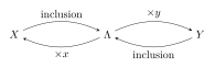
Reduction by the regular parameter gives a genuine exact diagram:
All three terms are -free, so the columns are exact and the free quotient prevents a Tor term in the bottom row. With generators on the two ends, explains the sign. This diagram is stronger than a drawing of four mesh diamonds with arbitrary rows and columns.
The lattice category is Frobenius. Alternating annihilator resolutions give
The embeddings above give enough injectives, and gives enough projectives. The projective-injectives are its finite free sums. Modulo them,
For example maps through give precisely inside . The two rows identify and . Hence its stable AR triangles are
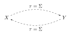
The four ordinary arrows through disappear in the stable category. A tube or a stable three-vertex grid would describe a different category.
For take the infinite closed algebra with chain vertices , endpoint loops , opposite chain arrows , and relations
Its single permitted cycle goes along the chain and back, with the endpoint loops. It is an actual sphere dessin: the Chebyshev map
has passport ; the dual contracted graph is a path. Its completed order has rank . Kill one arrow at every chain edge, retaining an orientation . The quotient is exactly of [116]. A surviving path has length at most , so the killed-arrow ideal contains . The polynomial algebra and its completion have the same finite quotient. Denote its intrinsic module category by .
For retain . The following table fixes all nine modules, not merely nine unlabelled points. A superscript denotes a formal inverse, not an inverse in the algebra. Each word is read in travel order; its basis consists of its successive visited positions.
| Label | word | start | dimension vector |
| 1 | |||
| 1 | |||
| 1 | |||
| 1 | |||
| 1 | |||
| 1 | |||
| 3 | |||
| 3 | |||
| 3 | |||
A direct letter sends the preceding position vector to the following one; an inverse letter sends the following vector to the preceding one. These rules satisfy and specify every arrow matrix.
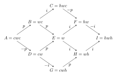
The maps are projections and embeddings. In the rectangular version, horizontal projections retain initial positions and horizontal embeddings append the final position. Upper vertical projections delete the initial , and lower vertical embeddings prepend . The signs in Figure 21.4 give
Their module intertwinings and exactness follow by these basis rules; for example the two maps out of have joint kernel zero, the maps to are onto, and the displayed dimension vectors give the kernel dimension at each vertex. The almost-split property is the additional content of the source’s hook/cohook theorem, after identifying as minimal of type .
Let mean left hooks when and left cohooks when ; let mean right hooks when and right cohooks when . These are operations on strings, not paths. Lemma 3.10 and the four-region induction in [116, Proposition 3.12] give every vertex of this component as
There are arrows increasing one coordinate at a time and
The meshes are
The nine labels are and the six intermediate positions. This is the whole component, continued in all four directions. Its two outgoing axis rays are monomorphisms and its two incoming axis corays epimorphisms. It is not an exact array of rows and columns.
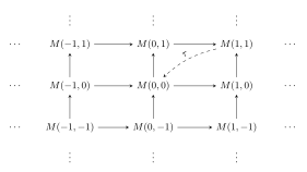
The complete module AR inventory is also known [116, Theorem 3.14]: one component containing the projective and injective modules; one exceptional tube of rank ; homogeneous band tubes; and the components above indexed by minimal type strings. In the exceptional tube has rank two. The source’s Figures 3–4 show the projective-injective component, not another view of this stable grid. None of these classifications is silently asserted for every module of the completed infinite order.
A short exact sequence gives a triangle in a bounded derived category, but almost splitness is tested against all objects there, including shifts. For a finite-dimensional algebra an indecomposable endpoint admits a derived AR triangle precisely when it is perfect; its translate is the derived Nakayama functor followed by . In the finite-dimensional gentle setting, [120, Section 5.1] applies this criterion to finite homotopy strings and bands, and describes the graded endpoint rotations. The finite-dimensional, grading, boundary and local-system hypotheses remain part of that theorem.
For our the failure of perfectness can be seen directly. In the travel/right convention the cover has the eight-element basis
and retains . Its kernel is . Multiplication by has kernel , since exactly the paths already starting with are killed. The terminal simple repeats through in the same way. Thus its minimal projective resolution has nonzero terms in arbitrarily high degrees. In particular the module AR sequence ending in in Figure 21.4 does not become an AR triangle ending in in .
By contrast, the smooth-support block of Proposition 21.4 is hereditary. The operator is a nonzerodivisor of the polynomial node algebra and its cokernel is , so it gives a length-one free resolution. The indecomposables in that block’s bounded derived category are ; each fixed shift has the same homogeneous tube and the AR triangles are induced by its exact sequences. The nodal stable lattice triangles above give another actual triangulated model. These two positive descriptions do not identify all of , and the stable lattice category.
Ringel’s is the tile of the five-bar wind wheel specified in [117, Section 12.5, p.30], drawn in Section 13.3, pp.38–40. It is part of an AR quilt, not just a finite-module mesh. Four finite-word quarters surround a nonperiodic two-sided word. The diagonals consist of one-sided limiting words; contracting ones use ordinary strings, expanding ones need completion, and the central mixed word needs partial completion. The five-tile example glues to a torus with five holes. Deleting the infinite-word points recovers its finite string components. This is a category construction, not an assertion that its quilt genus equals the genus of our original Belyi pair.
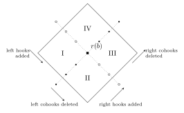
This picture is a finite-dimensional special-biserial wind-wheel category. It is not already our completed node or the quotient. No map identifying its algebra with a present dessin quotient has been supplied here. Such an import would have to specify that map and the category in which almost-split or pure-injective statements are retained. In particular deleting diagonals from one tile leaves four quarters, not one HLS grid. Ringel also lists indecomposable algebraically compact modules omitted from the quilt; it is not itself a classification of all ordinary modules or all pure-injectives.
Let , and . When the evaluated Hom map is square, chosen bases give
The action on coordinate functions has inverse weight. Put . The kernel is . If is the injective first map of a short projective resolution, its cokernel after Hom is and higher Ext vanish. A general presentation keeps its other cohomology. These distinctions are part of the semi-invariant construction, not consequences of an AR drawing [121].
Proposition 21.6 (A mesh whose determinant is a free generator). An actual dessin quotient has an almost-split mesh whose presentation semi-invariant generates a polynomial algebra with no relation.
Proof. In the Chebyshev order above kill vertex3, both loops and the reverse arrow, retaining only . This is the genuine continuous quotient . Its three indecomposables are and , by rank decomposition of a linear map. Its sequence
is almost split: a nonretraction to from these indecomposables factors through , and dually for . At dimension the single arrow coordinate transforms by . The short projective resolution gives the determinant . Its semi-invariant algebra is , with no algebraic relation among this one generator, although is a mesh relation. □
This quotient AR sequence is not ambient. A module supported at vertex1 with has a nonsplit epimorphism to . Every map from it to has zero vertex1 component, because while its own arrow is zero. That epimorphism cannot factor through in the larger category.
Proposition 21.7 (The product theorem with its hypotheses). Suppose is exact and have resolutions of length one by finite projectives. At a dimension vector where both end presentation Hom matrices are individually square, compatible bases give , up to the fixed basis sign.
Proof. Lift the projective cover of through . Its horseshoe kernel sits in a split sequence of the two projective kernels, so the middle resolution has differential . Applying contravariant Hom gives a triangular square matrix, with diagonal the two prescribed Hom maps. Its determinant is their product. □
Total squareness alone does not give the two factors. In the mesh at , has balanced Euler value, but and do not. The three individual Schofield factors are therefore not all defined there. Nor is the infinite-pd object eligible for the short-resolution hypothesis just because it sits in a diamond.
The lattice AR sequence of Theorem 21.5 is split after forgetting to . It therefore has the canonical line comparison
For any compatible endomorphisms it gives
| (21.3) |
Indeed an -splitting gives a triangular matrix. For every -linear endomorphism of , multiplication by , the basis makes that matrix and its two scalar actions explicit:
Both sides of (21.3) are . This is a determinant-functor statement after the specified passage to -perfect modules, not a nonexistent finite -projective resolution of . On applying the map between the first two -lines is multiplication by ; its cokernel is . Thus underived Hom is not exact on this AR row.
On the reduced continuous finite-length representation variety of the one-vertex node, the ordinary semi-invariant ring is in fact just . Scalar matrices act trivially by conjugation, forcing a nonzero character to have . The nilpotent filtration gives a one-parameter conjugation degeneration to zero arrows, so all invariant regular functions are constant. This coexists with the nontrivial lattice AR sequences and the relative determinant identity; the target data differ.
A genuine unframed relation is obtained by retaining both arrows , in a Chebyshev quotient and killing all other vertices and arrows. At dimension its coordinate ring is . The two coordinates have opposite torus weights and are semi-invariants. Their relation comes from the inherited zero relation; it was not deduced merely from a mesh picture.
For a richer example use the actual elliptic-square order. Its dessin has and ; there is one face, so gives genus one. The two quiver vertices are the two clean edges. The four arrows form one permitted alternating four-cycle, with two arrows in each direction; every mixed consecutive choice is forbidden. Put , set both reverse arrows to zero, and let the two forward arrows have arbitrary matrices . These modules kill and therefore extend continuously to the completed order. Frame the source : the acting group in the next statement is only . Write and .
Theorem 21.8 (A genuine framed generator relation). All six have target character , and their subalgebra is
The stated quadratic is the full ideal of relations of these six functions.
Proof. On the dense open , express the other columns in the basis and expand determinants. This gives the quadratic; polynomial continuation proves it everywhere. Conversely any nonzero six-tuple satisfying it is realized by four columns. After choosing a nonzero by permutation, one may take
Their last minor has the required value by the equation. The zero tuple is also realized. The quadratic is irreducible: its nondegenerate quadratic form has rank six, whereas a product of linear forms has rank at most two. Its ideal is prime, so this image description proves it is the kernel of the polynomial map on coordinate rings. □
The exact diagram behind decomposability is on the rank-two locus. Its exterior comparison relates complementary kernel minors. The relation extends to the lower-rank boundary; the diagram is not an almost-split sequence.
The framing is indispensable. With and , , but swapping the source basis makes it zero. Thus is not a semi-invariant for the full original source-and-target group. The coefficients of
are full-group semi-invariants. The framed six-generator relation must not be misidentified as their unframed presentation.
The chapter supplies exact categories, explicit maps, parameter spaces and some genuine determinant identities. These can organize an effective model’s states and couplings, but is a categorical translation, not by itself a unitary time evolution or a self-adjoint Hamiltonian. A physical realization must supply its Hilbert space, domain, positive metric and dynamics independently. Likewise an arbitrary tube parameter is not a prime norm or a Frobenius eigenvalue.
A valid route from a mesh to polynomial functions requires a universal family, the correct group action, determinant-admissible complexes and rank hypotheses. A route from those functions to an arithmetic -function additionally requires descent, local factors, conductor and archimedean data, convergence or regularization, and a determinant-preserving positive comparison. The relative nodal identity and framed Plücker model give usable intermediate constructions. They do not discharge those arithmetic or analytic obligations, and no full GRH conclusion is asserted.
The new covering calculation in Section 7 is useful for computations, precisely because its limitations are explicit. The parent algebra is our infinite elliptic theta algebra, its truncation is a finite quotient, and its cover has vertices indexed by integers. They are three different categories. The nine-dimensional module in Proposition 7.2 and the higher-genus family in Corollary 7.3 show that even this genuine covering does not reach every module or bounded derived object.
The lecture [74] supplies the covering language: locally bounded categories, exact push-down/pull-up and graded adjunctions. Its Theorems 4.23 and 4.28 give precoverings on the specified module and bounded derived categories. The AR-quiver covering theorem 4.18 assumes an actual Galois covering between Hom-finite Krull–Schmidt categories; density cannot be dropped. A universal bound-quiver cover also depends on its relations and presentation. It is not automatically a covering of the compact surface.
The GLS paper [75] works over an algebraically closed characteristic-zero field. Its finite-dimensional GLS algebras are not automatically our surface orders. Equivariantization transports string/band information to certain non-string algebras. Theorem B includes , and tube components, with its stated indexing. Theorem C corrects a naive root-only prediction by the additional rank vectors in the named tame affine family. Here vertexwise local freeness and its rank vector concern the GLS vertex algebras; they are not freeness over the central DVR of a surface order.
Schroll’s survey [76], particularly Sections 4–5, organizes graded gentle categories through curves, local systems, crossings and twisted complexes, with grading encoded by a line field. Its framework distinguishes perfect objects from finite-total-cohomology objects, and properness from homological smoothness. These distinctions matter for our infinite algebras and for any completed or operator-algebra version.
At finite the cover is locally bounded: only lengths below survive. Without the cutoff, each vertex has infinitely many nonzero outgoing Hom spaces, so the locally bounded hypothesis used above fails. Locally finite dimensional Hom spaces alone do not repair that failure. Conversely the truncated algebra has extra length relations and is not entitled to all quadratic-gentle surface-model theorems.
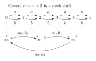
Mixed paths and all paths of length vanish on both rows.
The dotted lines are the residue map, not irreducible module maps. The top row is a finite window of the quiver of the cover, not an AR component. The proof of the Hom decomposition, the unequal Hom-control defects and the full nine-dimensional calculation appear in Sections 7 and 20; they are not inferred from the drawing. The genus-four instance has dimension 27, and the genus-nine instance dimension 57, with the same exact lift obstruction.
The branch swap preserves . Thus it acts on and defines the skew-group algebra . An equivariant object needs an isomorphism satisfying the cocycle equation . A fixed isomorphism class alone does not choose . For the nine-dimensional witness, the unequal branch ranks rule out even ; the induced pair instead has a canonical swapping action. This is a concrete use of equivariant machinery without asserting a GLS identification or drawing a folded AR component whose almost-split property has not been checked.
Let be the compact objects of and write for finite-dimensional total cohomology. For our infinite zero-graded , its regular projective is perfect but has infinite -dimension; hence it does not belong to . This is already a counterexample to silently embedding the former category in the latter. In proper smooth finite-dimensional situations the familiar equivalences have stronger conclusions; these hypotheses cannot be omitted here.
A curve model must retain the dissection, stops or punctures, line field, intersection grading, local systems and dg or enhancement. For perfect complexes, the finite deck decomposition of the Hom complex is proved in Section 20. For a matrix of paths representing a differential one must still check ; intersections without degrees and composition data do not prove this identity. A marked surface used for the Fukaya model is not automatically the original compact Riemann surface with its analytic metric and all boundary data forgotten.
Completion to requires continuous modules and the chosen topology. The finite quotient modules extend continuously because a power of annihilates them. They are not central-DVR-free lattices: in the nine-dimensional example the central length-three parameter already acts by zero. The cutoffs must not be renamed .
For a useful arithmetic determinant, these categorical constructions still need a prime correspondence, a perfect or analytically controlled target, a determinant-line comparison, conductor and archimedean normalization, and positivity for that same arithmetic function. A derived equivalence or an AR translation does not supply a Hilbert-space adjoint, self-adjoint domain or trace-class convergence. These remain the spectral program’s independent load-bearing obligations.
The executable calculation is examples/coverings/theta_cover.py. The exact matrix obstruction is checked in lean-analytic/CoveringBand.lean. The latter verifies selected actual matrices, not every category or equivalence discussed here.
For a finite-dimensional quotient, a specified projective presentation can define a determinant semi-invariant by applying , provided the resulting vector spaces have equal dimension and bases or determinant lines have been fixed. The covering Hom decomposition makes this matrix computable by deck components; it does not make it block diagonal. Cross-degree terms matter. Already
differs from the product of its two diagonal entries. A product over deck blocks is justified only after proving that the relevant differential or endomorphism preserves those blocks. AR mesh relations concern morphism compositions; a presentation of a ring of semi-invariants requires additional generation and relation proofs, as in the earlier determinant chapters. Neither the GLS root lattice nor a surface intersection form provides the missing positive Hilbert inner product or arithmetic factor identity by itself.
This chapter develops original 2053 lines 1097–1307 on the genuine infinite dessin algebra, correcting the graph and category conventions before using them in a determinant calculation. The finite module category is specified inside the infinite algebra; a finite diagram is not substituted for that algebra. The companion exposes every kernel/image dimension, the branch monodromy and its polynomial-versus-completed-order status.
The original linear-relations chapter mixes graphs, partial relations and stable kernels. We keep these different objects separate. For a field , a linear relation is a subspace ; its inverse swaps coordinates and . The full graph always has dimension , including pairs with zero output. In particular , whereas . Thus the source’s is zero, not the ordinary stable kernel.
For odd , use the actual clean dessin of , , on the compact smooth curve, in characteristic zero. Its genus is ; its infinite locally gentle algebra has vertices , arrows , and mixed consecutive branch products zero. Below paths act in their direction of travel on left representations over any coefficient field . Let be the full category of finite-dimensional representations with every and invertible for .
Theorem 23.1 (A concrete relation category on an infinite dessin algebra). The category is equivalent to finite-dimensional pairs with intertwining maps. A normal form puts at each vertex, , and all other . For ,
These summands and their kernel/image filtrations are functorial. The first restriction is nilpotent and the second invertible. The central full-turn parameter acts as . A finite extends continuously to the -adically completed order precisely when is nilpotent. Such modules are torsion, not nonzero order lattices.
Proof. Transport all vertex spaces to vertex zero along the invertible arrows; the remaining map is the full-turn monodromy . Arrow-compatible maps become exactly . Finite kernel/image chains stabilize by step . If and , then , hence ; rank-nullity proves the direct sum. Stability gives the two restrictions, and proves functoriality. Continuity on a finite-dimensional discrete space means some kills it. Conversely nilpotence makes every formal series act by a finite sum. This proves the completion assertion. □
Over an algebraically closed , the indecomposable branch pairs are . The value is permitted for a polynomial band; it is not a forbidden deformation parameter. The nilpotent blocks are strings, but are not all rigid: is a nonsplit self-extension of . The Hom dimension between two such Jordan pairs is for equal eigenvalues and zero otherwise. These assertions concern this specified full subcategory, not all infinite modules.
If transports once along the -arrows on , then
| (23.1) |
Eliminating the identity arrow blocks leaves the final monodromy block; the eliminated identity blocks have determinant one. For the answer is . Nilpotent strings therefore contribute one, and arbitrary bands have no forced unit-circle zero location. This determinant is an actual cyclic-quiver invariant; it is not the missing arithmetic positive determinant comparison.
In the original basis let , , and , , . Then
Each graph has dimension three. Omitting zero-output generators changes the relation into a partial graph and changes its powers and domain. The following are subspaces of , not lists of pairs in :
For all four full graphs . This corrects both the source’s graph convention and its interchanged kernel entries. For an arbitrary multivalued relation there need not even be a linear map on its domain; its regular-part theorem requires the appropriate relation subquotients and finiteness conditions. We do not replace those hypotheses by the graph calculation. For comparison, in [38, Section 4, Lemmas 4.2,4.5–4.6] write and let consist of vectors with a compatible infinite backward chain. In finite dimension ; this equality is not automatic for arbitrary infinite-dimensional spaces. The regular quotient is , where
The automorphism statement uses this quotient for an arbitrary relation. The splitting statement additionally requires its finite-dimensionality, rather than the source’s unqualified expression.
Write for and , with ; the rightmost map acts first. Every is an isomorphism. Conjugating the arrow maps by these identifications makes for , and makes at the remaining arrow. All -relations vanish. An intertwiner is transported to maps with for and . Hence every and . This proves full faithfulness and essential surjectivity, with inverse given by . It is also an exact equivalence: kernels and cokernels of intertwiners are the usual invariant kernels/cokernels; the identity arrow maps remain identities. Finite dimension is a condition on modules, while itself is infinite dimensional through its arbitrarily long permitted branch paths.
The sum of the full permitted turns on both branches is central in this closed dessin algebra. On the chosen modules the -turns vanish and each -turn equals , so acts as at every vertex. If , the action factors through and extends to the completion. If has a nonzero invertible Fitting summand, no power of kills that summand, precluding continuity. For with , the obstruction is stronger: is a unit of but its th power annihilates the proposed module, impossible for a nonzero unital module. This rules out even an unqualified algebraic extension of that band, not just a chosen topology.
Kernel dimensions are nondecreasing and at most . Once two successive kernels agree, applying shows that all later kernels agree. Thus they stabilize by ; rank-nullity gives image stabilization as well. On , . On , ; finite dimension makes this a bijection. If , induction gives , hence
This proves functoriality even when : choose a common stabilization exponent for the two finite objects. The decomposition projection onto along is canonical and commutes with all intertwiners; the existence of a Jordan basis is not needed. Finite dimension is essential. On , multiplication by has stable kernel zero and stable image , although . The same construction is an actual infinite-dimensional module of . Thus the finite Fitting split cannot be extended to every module of our infinite algebra merely by repeating its notation.
Let , with , and form . For a nilpotent Jordan block of size , , so counts the blocks of size at least , and counts blocks of size exactly . For the stable dimensions are and ; the kernel dimensions begin . The are functorial subquotients. Their dimensions do not specify a natural choice of basis or split each filtration step.
Proposition 23.2 (What the source’s splitting-functor assumptions imply). Let be additive categories with finite biproducts. Suppose additive functors and satisfy , for ; only finitely many are nonzero for each ; the jointly reflect isomorphisms; and maps have invertible -images. Then . Every nonzero indecomposable is for a unique index and an indecomposable up to isomorphism.
Proof. Sum the finitely many nonzero to a map . After applying , all off-diagonal summands vanish, leaving the assumed isomorphism , or . Joint reflection therefore makes invertible. For an indecomposable , exactly one of the nonzero summands can occur. Conversely, if and is indecomposable, applying makes one summand vanish, say ; every other also vanishes. Joint reflection applied to gives up to isomorphism. Finally apply to an isomorphism to recover both index and object. □
The direction of matters: it is into , contrary to one source diagram. Local finiteness is objectwise in , not a finiteness assertion over all objects of a category. Abelian categories require kernels, cokernels and the usual exactness axioms; addition is on Hom groups, not on an alleged group of quiver vertices. The abstract assumptions above do not assert that the family is faithful on arbitrary morphisms. Our Fitting example is concrete: consists of nilpotent pairs, of invertible pairs, are inclusions and the two stable summands.
In this branch category, Jordan normal form classifies indecomposables over an algebraically closed field. Over a general field replace Jordan eigenvalues by powers of monic irreducible polynomials. A Jordan block is one directed string with basis visits and nonzero successor arrows; for is a permitted cycle band. Formal inverse letters are reverse traversals, not inverse elements of . Strings and their reverses describe the same string module under the usual isomorphism convention. Arbitrary infinite modules are not all classified by this finite calculation; the actual finiteness hypotheses in [38] remain essential.
Identify a Jordan pair with . An intertwiner from size to size is determined by the image of , annihilated by . For equal eigenvalues this subspace has dimension . For different eigenvalues, Bezout’s identity makes invertible on the target, so only zero remains. Full faithfulness above transfers this Hom computation to . The sequence is not split: with , a lift of the quotient generator has nonzero first coordinate and is not killed by . Its image under is a nonsplit ambient- self-extension. Thus even the string is not rigid. No assertion that this exact full subcategory is derived fully faithful is needed for the nonsplitting argument.
For this particular closed , every oriented or inverse letter has exactly two admissible successors: continue on its branch in the same orientation, or switch branch and reverse orientation. Cancellation and forbidden pairs, including inverse forbidden pairs, remove the other choices. A fixed ordering of these choices identifies each first-letter cylinder with . The whole infinite-word space is a finite disjoint union of Cantor spaces, hence itself Cantor. There are no terminating words inside that space to remove. Arbitrary gentle quivers can have isolated or eventually forced paths, so this conclusion is not universal. Algebraic covers retain the lifted zero-relations and deck equivariance data; arbitrary periodic cover representations are not automatically bands or a unitary time evolution.
On , . For a direct determinant proof of (23.1), successively eliminate the blocks at vertices in . Block row additions preserve determinant and leave at vertex zero. This works over without inverting or ; the zero-size case gives one on both sides. The Fitting splitting separates a nilpotent factor and the determinant on the invertible summand. For instance , gives , whose complex roots have modulus , despite being a genuine genus-two dessin module.
Under conjugation of this is an invariant polynomial. With independent source/target bases a presentation determinant is instead a semi-invariant with its determinant-character weight; those actions must not be conflated. The polynomial equality does not construct a positive Hermitian metric, an arithmetic Euler factor, a regularized determinant or a zero-preserving map to completed -functions. Functorial kernel filtrations similarly do not construct an equivalence of derived/Fukaya categories. A fixed graded surface category and a determinant-compatible arithmetic realization remain separate obligations.
The exact rational checker evaluates actual genus-two/four quivers, Hom equations, full-turn matrices, both filtration directions and the nonsplit extension. lean-analytic/LinearRelations.lean proves full graph identities, semiconjugacy and filtration preservation, actual finite-space Fitting splitting/stabilization and unit-power annihilation. It does not package the entire dessin category, Jordan classification, general splitting-functor proposition or determinant proof in Lean.
The preceding branch example can be realized on every element of the infinite algebra, rather than verified only on sampled arrow matrices. Use the complex genus-two clean dessin , , and any coefficient field . Put equal to the matrices whose reduction modulo is upper triangular. Let
where each map to takes the constant diagonal. Equivalently, is generated inside by
Indices are modulo five. Matrix multiplication acts on left column modules. The path-normal-form proof below identifies with ; this is a polynomial algebra, not an arrow-truncated finite quotient.
Theorem 23.3 (An ambient module extension). Let , and . For , act on by and on by . These are unital -modules, and
is exact and nonsplit. Moreover is infinite dimensional over . The assertions hold in every characteristic, including two.
Proof. Evaluation of polynomials gives both actions. Multiplying proves -linearity of ; their kernel and image follow coordinatewise. If were a -linear section, the constant coefficient of would be one. But kills , while has nonzero coefficient, a contradiction. Finally the permitted turn has first component . The unital algebra map , , is injective: its first-component entry is . Thus cannot be finite dimensional. □
In the preceding notation these modules are and . They are finite torsion modules over an infinite algebra; they are not nonzero lattices over its completed surface order. The nonsplit sequence defines a nonzero Yoneda extension class in the ambient module category. No assertion that it is almost split in that entire category is needed or inferred. In particular it does not supply an arithmetic spectral determinant or a zero-location theorem.
Theorem 23.4 (Unbounded normal-image faithfulness). In , index the stationary images by and the positive images by , where , , and or . The positive image is in factor , with zero in the other factor. Its path length is . All these images, including the shared stationary images, are linearly independent over every field. Every finite normal expansion has uniquely recoverable coefficients, without a bound on degree or path length.
Proof. Read a stationary coefficient from the first factor’s constant diagonal; read a positive coefficient from the indicated factor, entry and degree. The index restriction ensures that no positive image contributes to a constant diagonal. These linear selectors are biorthogonal to the images, so applying each selector to a finite expansion recovers its coefficient. □
This theorem is now kernel checked for actual polynomial matrix pairs. The membership and spanning steps are supplied by the next theorem. Comparison with a separately constructed path quotient remains a distinct algebraic formalization task.
Theorem 23.5 (Normal coordinates in the generated algebra). Let be the algebra generated by the displayed vertices and arrows, and let be the normal index set of Theorem 23.4. Every normal image belongs to . The actual -valued finite expansion
is a linear isomorphism, whose inverse is . Thus the normal images form a basis of the infinite generated algebra, not merely an independent family in its ambient matrix space.
Proof. Write for the shortest positive branch walk from to , using a full turn when . Its image is in branch , where if and otherwise. The actual arrow product has image for every . Admissibility gives , so proves membership.
The normal span contains the generators and and is multiplicatively closed: stationary factors select endpoints; positive factors either multiply to zero or to in the same branch. When , the two strict upper inequalities imply , so this output slot is still permitted. Adjoin induction gives spanning of . The previous coefficient selectors prove uniqueness and the inverse formula. □
All membership, spanning and finite-expansion assertions in this theorem are now Lean checked over arbitrary fields. The formal linear equivalence is not asserted to be an algebra map from an independently defined path quotient, nor a statement about completed orders, derived categories or GRH.
With our convention a path from to acts as ; the rightmost arrow acts first. Every nonzero positive path uses only the -branch or only the -branch, because mixed consecutive arrows are the defining quadratic zero relations. Along either branch the path of length starting at is unique. Write
Its image is in the chosen factor and zero in the other. For , ; for , ; for and positive length, . The stationary path is the shared .
These images are linearly independent: off-diagonal matrix units, positive diagonal monomials, branch factors and degrees are independent; the shared constant diagonal units are independent of all positive paths. They span , since upper entries permit all polynomials, lower entries are divisible by , and only the constant diagonals of the two factors must agree. Products of paths agree with matrix products. Thus the arrow assignment induces a bijective algebra map from to . This argument includes arbitrarily long paths; it imposes no nilpotence relation on a full turn.
The central parameter , the sum of all full turns on both branches, has image . Completing in this parameter is a separate operation. The polynomial algebra and its completion are not identified by the normal-form calculation. The finite modules below are annihilated by , so their continuous completed actions require only a finite Taylor polynomial.
Here is an explicit proof of Theorem 23.4 and the coordinate convention used by the implementation. Let
For a stationary index set ; for a positive index set and . These are elements of the ambient polynomial matrix-pair space, with no degree cutoff. For define
Here the subscript in the second formula denotes either branch. Every is -linear, since extraction of a fixed matrix entry and polynomial coefficient is linear.
We verify , including the cases at degree zero. For two stationary indices this is the ordinary diagonal matrix-unit identity. A stationary selector vanishes on a positive image in the other factor. In its own factor it could see a constant diagonal only if and , which the definition of excludes. Conversely, a positive selector applied to a stationary image could be nonzero only at precisely the same forbidden slot. For two positive indices, different branches have disjoint supports. In one branch the matrix entry forces both endpoints to agree and the monomial coefficient forces the degrees to agree. These conditions give equality of the full indices. The witness of the condition defining carries no extra algebraic data. This proves biorthogonality in every characteristic, using no division.
For any finitely supported , linearity now gives
If the sum vanishes, every vanishes; if two sums agree, their coefficients agree. This proves linear independence and injectivity of normal expansion on the actual -module of finitely supported functions. It does not replace finite support by a convergent or formal infinite sum.
The length formula also contains useful information beyond independence. If then even at ; otherwise and give the same strict inequality. Hence is a positive integer, and . For fixed starting vertex and length , two such equations imply . Since , this forces and then . In Lean the subtraction is natural subtraction; positivity is proved before using the rearranged equation.
For example the -path of length from vertex ends at vertex and has image . The length- -path from to has image . Their product, with the rightmost path first, is , of length . Replacing the second path by its -branch version makes the product zero. Degree-zero upper entries such as are permitted, but is not a stationary image: the stationary element is the shared pair . This last distinction prevents a spurious extra idempotent in the proposed basis.
The selector theorem alone gives the faithfulness part of the intended quotient comparison. The next construction proves membership and spanning inside the generated algebra without assuming that comparison. A separately defined path algebra, mixed-zero quotient and its universal algebra map still require formal packaging. Completion, module-category and almost-split universal properties require their own subsequent constructions. None of these finite-support identities supplies an arithmetic self-adjoint determinant or controls zeta zeros.
We now prove Theorem 23.5. This closes the membership and spanning gap left by ambient coefficient recovery. Let modulo five and, inside the actual generated algebra, define
In this formula denotes the arrow in the chosen branch; it may be an -arrow. The rightmost arrow acts first. This recursive definition is an element of for every , because it uses only its generators and multiplication. Set
The integer lies between one and five. In particular is a positive full turn, whereas is the shared stationary idempotent. These two elements are not interchangeable.
Directly following the arrows, the path crosses the weighted arrow exactly times. Its image is therefore in factor , with zero in the other factor. The Lean proof checks all five-by-five endpoint pairs for each of the two branches; this is a finite verification of a finite combinatorial case split, not a bound on permitted path lengths. For all , induction gives
For the power is the unit of the whole two-factor algebra, so multiplication by still selects the correct branch. The induction step uses with image and . No assertion that a branch-only degree-zero diagonal belongs to the algebra is needed. Since a permitted slot satisfies , the choice constructs its preimage in . This proves membership at every polynomial degree.
For clarity, if , , , then and realizes by a length- arrow word. For , , , we have and the exponent is zero. The corresponding exponent must never be replaced by a negative power or by an inverse arrow. The construction works over as well as characteristic zero.
Let be the -linear span of all normal images in the ambient space. Membership just proved gives . We prove the reverse inclusion by showing that is closed under the operations used to generate . The product rules are
and for two positive images
The displayed nonzero output is always an admissible positive image. If this follows from its degree. If , nonnegativity gives , so the input conditions imply . Thus and the output is admissible even at degree zero. This explains why closure cannot be justified merely by ignoring the lower-triangular constraints.
By bilinearity the product of two finite linear combinations lies in . Every vertex is one of its normal images, and each arrow is a permitted image with degree zero except the wrap arrow, which has degree one. The sum of the shared vertices is the unit. Scalar multiples of this unit belong to . Induction on the algebra generated by the arrows and vertices therefore gives . In Lean this is actual Algebra.adjoin_induction, not a predicate that assumes the desired normal form for every element. Consequently as submodules of the polynomial matrix-pair space.
Now lift each to an element using its proved membership. Their images under the injective inclusion are the already independent ambient images, so the lifts are independent. The equality gives surjectivity of finite expansion; independence gives injectivity. This constructs the linear equivalence on the genuine generated algebra. For any , apply the ambient coefficient recovery identity to to obtain
The formula holds for every element of , not only on a sampled list of paths or generators. Its finite support follows from the equivalence with finitely supported functions. No convergence of an infinite expansion is asserted. Although the product table has been used to prove span closure, we have not yet supplied the formal universal map from a separately constructed bound-quiver path quotient. The distinction between a linear coordinate equivalence and that algebraic quotient interface is retained.
In coordinates let be the first component of an arbitrary -element. Its action is
Evaluation is multiplicative: the constant coefficient of a product is and the linear coefficient is . Consequently the formula is a representation of the entire algebra. The second branch acts by zero but has not been removed from the algebra. Both maps in the sequence commute with this general block action, not merely with a finite test list of generators.

Every vector in is , is injective, and is surjective by . The section obstruction uses only : it is zero on , while on it sends the coordinate-zero constant coefficient to the coordinate-four infinitesimal part. A section commuting with this arrow would force . No algebraic closure, eigenvalue classification, division by two or positivity premise occurs.
The file lean-analytic/BranchExtension.lean defines as the actual generated subalgebra of polynomial matrix pairs, proves its infinite dimensionality through injective polynomial evaluation, and constructs as -linear maps. The original 21 printed theorem types and axiom reports cover the generators, infinite embedding, actions, exactness and absence of a module section. Eight additional reports in NormalPath cover slot extensionality, positive length, the length equation, recovery from start and length, biorthogonality, coefficient recovery, linear independence and injective normal expansion. Ten further printed reports now establish actual generated-algebra membership, equality with the normal span, lifted independence, bijective finite expansion and its explicit inverse coefficients. The normal-form isomorphism with the separately constructed path quotient above is proved in prose; it is not packaged as a Lean categorical equivalence. Nor is a Yoneda-Ext object or the universal factorization property of an almost-split sequence formalized by these maps alone.
The exact checker examples/relations/check_extension.py independently uses unbounded normal paths and polynomial matrix pairs. It checks 405 distinct paths through length 40, 7,225 products, 30 distinct loop powers and 80 whole-polynomial module actions. The full generator system for a hypothetical section has coefficient rank 49 and augmented rank 50 over . These finite diagnostics complement the symbolic proof; their finite cutoffs do not establish infinite dimensionality by themselves.
The separate exact checker examples/relations/check_normal_paths.py checks 475 normal images at degrees up to (length ), all 225,625 selector pairs, 1,030 direct arrow steps, 15,625 composable-or-zero product comparisons and 200 finite expansions over . Invalid constant slots are rejected. These are finite diagnostics of the code and conventions; the unbounded assertion is established by the Lean theorem, not by the size of the tests.
A further deterministic checker, examples/relations/check_normal_algebra.py, constructs all 50 shortest arrow words and 375 actual preimages, including degree , using sparse binary powers of the full turns. It checks 5,625 product round trips and 200 exact expansions over the four stated fields. Three ambient matrices with forbidden constant shapes fail reconstruction, as required. These diagnostics test the implementation independently of finite degree bounds; the general membership/span/equivalence result is the Lean theorem, not an extrapolation from these samples.
A derived construction begins with a differential and its cohomology, not with a proposed physical clock. This chapter develops the DG material of the original 2053 manuscript, lines1308–1478. Throughout this chapter is a field. We use the actual infinite nodal and theta dessin algebras. The source is preserved unchanged. Its unit-boundary example and self-extension count require corrections; its higher-product and physical interpretations require explicit additional data.
We use cohomological grading. A unital DG algebra is a graded algebra with , and on homogeneous elements. A DG map preserves multiplication, the unit, degrees and the differential. It is a quasi-isomorphism when it induces isomorphisms on every cohomology group. A left DG module has the corresponding Leibniz rule for its action. The exterior generator’s degree must be declared; the notation alone does not specify negative degrees.
Proposition 24.1 (A unit boundary is contractible). If satisfies , the underlying -complex of every unital left DG -module is contractible. In particular ; it is not a DG resolution of a nonzero field with zero differential.
Proof. Define by . Then , so . Every cocycle is therefore . For a right module the correct formula is : its two compositions have opposite terms and again sum to . Taking the regular module proves the algebra assertion. The displayed homotopy is -linear; graded -linearity would require an additional compatibility, such as graded centrality of . A unital chain map to a nonzero field would send both to zero and to one, which is impossible. □
The qualifier is essential for a general noncommutative DG algebra. Over our actual nodal algebra , let in degrees and with commutator differential. The inverse-arrow homotopy satisfies . But a degree- graded -linear endomorphism of must commute with the even projection onto ; its only possible component is then zero. Thus is acyclic and its underlying complex contracts, without being contractible by a -linear homotopy. Derived and homotopy categories must not be conflated.
For the source’s two-piece example , the differential is the identity . Both cohomology groups vanish. The auxiliary identity for a Koszul relation is useful instead of assuming nonzero cohomology [78].
The clean interval dessin on the sphere gives , with basis . It remains infinite dimensional. The variables here are actual dessin loops; they are distinct from the auxiliary persistence parameters used later in the book. Set and consider
The product is ordinary coefficient multiplication, with and commuting with degree-zero coefficients. The odd square relation is imposed also in characteristic two. Proposition 2.5 proves all Leibniz cases and the cohomology. Explicitly, writing and gives
This sign formula extends the homogeneous rule linearly; is not an ordinary ungraded derivation of this commutative square-zero algebra.
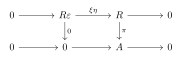
The diagram compares cochain degrees . The map is quotient augmentation, not an inclusion of into . Its kernel is , and multiplication by is injective since is a domain. Thus the cohomology comparison is an isomorphism in every degree. The two ambient terms are free over . They are not asserted to be free -modules: the nonzero element acts on them, so their action does not even factor through . This DG replacement does not shorten the infinite projective resolution of a nodal residue simple over .
For an explicit calculation, , whereas and survive in . A polynomial has a unique normal form , where ; remove every monomial divisible by . Their linear independence follows by setting each variable to zero. This identifies the quotient with the polynomial branch pullback.
Write . The same two-term construction over maps to
Here is a coefficientwise proof, avoiding an unjustified interchange of completion and arbitrary cohomology. The branch-evaluation map sends to . Every equal-constant pair is the image of . Its kernel consists of series whose coefficients on both coordinate axes are zero. Such a series is uniquely by shifting both exponents down one. The same shift proves multiplication by injective. Consequently the completed Koszul model has , and no other cohomology. All these maps are continuous for the maximal-ideal topologies: evaluation preserves powers, and the product relation raises order by two. This is the actual completed surface order already used in the node chapter.
An isomorphism by itself is not this result. For example , , , , has the same and nonzero . Projection to is not a quasi-isomorphism. A DG enhancement must specify the DG map or a justified zigzag and prove the required cohomology comparisons. Equivalences of derived DG-module categories use an external change-of-algebra theorem with its hypotheses; they do not follow from a single ordinary algebra isomorphism on .
For , define , . Substitution is a polynomial algebra automorphism, inverse to , and fixes . It acts coefficientwise on , fixing , so
Multiplicativity follows from the two-piece product formula. The completed substitution preserves each maximal-ideal power, so extends continuously, with continuous inverse, to the formal DG model and branch pullback. It is a semilinear chain automorphism over the ambient coefficient ring: , not generally an -linear map.
The diagonal DVR , , has branches . The clock sends to the pair . If this is a diagonal series , its two linear coefficients must agree; hence . Conversely, if , substitution sends to and preserves the diagonal subring. It fixes that subring pointwise exactly when , as the image of shows. In characteristic two these alternatives may coincide. Thus preserving the relation and order topology does not by itself preserve a chosen fixed coefficient action.
For and , the coefficient of acquires phase . A selected finite monomial space with its declared orthonormal basis then has a unitary diagonal action. Choosing that finite norm does not construct a canonical Hilbert completion of the order, a self-adjoint arithmetic generator or an -function comparison. The positive-transfer and unitary-logarithm distinctions in the physics chapters still apply. Gluing DG clocks further requires actual compatible maps and coherences; no gluing theorem is inferred here.
The source calls its double-three-cycle example spherical. Keep that rational theta distinct from the elliptic theta. Both have , but their dart involutions are respectively and . Write vertices as the sorted -pairs ; for the elliptic case these are . The simples are the residue simples of the actual infinite dessin algebra. The exact forbidden-word resolution of Theorem 2.1 has two positive-degree arms. After Hom to a residue simple, every arrow differential vanishes, so Ext dimension counts the terminal vertices of these arms, not just arrows leaving the initial vertex.
Proposition 24.2 (Two different Ext tables). For the dimension matrix is the identity. For , using right-module and path-travel conventions of the resolution chapter, the elliptic theta has
For the spherical theta, positive even give on the diagonal and zero elsewhere; odd give zero on the diagonal and at each other vertex.
Proof. For the elliptic involution, both initial arrows lower the vertex label by one modulo three; every next forbidden arrow does the same. Hence both length- indexing words end at . For the spherical involution the forbidden dart permutation has cycles . Each two-step arm returns to its initial vertex, while its first step reaches one of the two other vertices, one arm each. This proves all positive degrees; degree zero is Hom between pairwise distinct residue simples. Minimality of the exact resolution supplies the Hom differential vanishing already used above. □
Thus neither example has two-dimensional self . The two self-extension tables are
These are module Ext groups, not stable AR arrows, finite-cutoff quotient Ext groups or an asserted surface-intersection classification. The completed residue-simple calculation follows the earlier formal-series resolution; other continuous-module and derived equivalences need their own arguments.
For an uncurved cohomological algebra, has degree . With the graded tensor sign convention its identities are
When , the identity makes associative. The operation is therefore not its ordinary associator. Minimal-model existence over a field and the appropriate derived comparison are external results of Keller [77, §§3.1,3.3,6.2]; they are not formalized here. For an ordinary algebra concentrated in degree zero, taking to be its product and all other operations zero already gives a minimal model. For our nodal DG resolution the cohomology is likewise concentrated in zero, so every higher , , has zero target by degree. This model therefore supplies no compulsory nonzero higher operation or physical curvature.
The Ext algebra of a sum of simples is a different graded object. To build its derived composition data, choose an appropriate projective resolution and use the DG endomorphisms with . Expanding twice cancels the mixed terms and leaves . Bounded-above projective resolutions in the ordinary module category give the familiar derived-Hom model; completed and topological versions must specify their Hom spaces and admissible maps.
There is also a useful grading test. Suppose an Ext minimal model is diagonal in cohomological/internal degree and its operations preserve internal weight. On inputs of cohomological degrees , has output degree but internal weight . Diagonality forces unless the output vanishes. The polynomial quadratic-monomial theta resolutions are linear, so their Ext has this diagonal grading. A transfer using contractions chosen separately in each internal weight over a field retains it. Thus an internally compatible model can have every higher zero. This statement concerns that graded polynomial interface; it is not an identification of all ungraded or completed enhancements, nor an assertion that an arbitrary numerically fitted operation is a minimal model. No physical curvature or arithmetic positivity follows from the symbol .
The graded enveloping algebra is with Koszul signs; Hochschild objects are the derived tensor and derived Hom , with their homological or cohomological conventions declared. Derived base tensor or flatness is needed beyond the field setting. Completed continuous Hochschild theory also requires its completed tensor and continuity conventions. These objects are not interchangeable with an arbitrary ordinary matrix trace.
For the ordinary commutative nodal algebra, one concrete calculation is : the degree-one Hochschild boundary sends to . This quotient of the infinite-dimensional algebra carries universal trace classes but chooses neither a functional nor a positive state. Over declare self-adjoint and conjugate coefficients under . The origin evaluation is a clock-invariant positive state, since . Its negative is still an invariant trace but is not positive, as its value at one shows. Even the positive choice has GNS null space , so its GNS Hilbert space is just . This follows directly from the displayed seminorm, and shows that trace classes, positivity and a useful spectral representation are three separate choices. No arithmetic determinant is obtained here.
A strict filtered DG module is a functor from a poset: its maps preserve degrees, actions and differentials, identities are identities, and every comparable triple has exactly the same composite map. A homotopy-coherent replacement must supply the higher coherences too; pairwise homotopies alone do not define it. For an actual example over our nodal DG model,
forms a family of DG -submodules, with inclusion maps when and . Indeed multiplying by the central degree-zero monomial commutes with , and these ideals are closed under the -action. Inclusions compose literally; the clock preserves each ideal up to its scalar . Componentwise divisibility also gives . This is a decreasing module filtration indexed with the declared reversed order.
The declared involution also matters. For self-adjoint , a nonreal phase makes an algebra automorphism which is not a -automorphism. If a unitary implements it in a -representation and is self-adjoint, then is self-adjoint, so and hence ; the same holds for . Thus this particular nonreal clock cannot act faithfully by unitary conjugation with those self-adjoint branch conventions. This does not exclude other involutions or graph-operator constructions with different adjoint generators; it forbids silently identifying their adjoints with these declared ones.
The finite monomial windows below instead form increasing subcomplexes of -vector spaces. They are not -submodules or DG -submodules, because multiplying by a variable leaves the box. Inverting both variables to manufacture increasing fractional modules would make a unit: then and the localized DG algebra contracts. Such localization loses the node rather than improving its derived resolution.
The remaining source interfaces need their own constructions: bar/cobar, Ginzburg and Fukaya enhancements are not selected by merely matching ; gluing up to homotopy requires coherent maps. Nor does a symbol identify a Hochschild deformation or a measured curvature. The existing unitary-logarithm discussion is retained in the physics chapter. Its nonunitary counterpart needs care: a singular finite matrix cannot be an exponential, since every matrix exponential is invertible. An invertible unipotent matrix has a finite nilpotent logarithm in characteristic zero, which is not a self-adjoint generator unless the matrix is the identity. These observations delimit the operator interface without assuming a physical realization of the algebraic clock.
The canonical laboratory shows a finite subcomplex, not a finite parent algebra. For it retains source monomials and target monomials . Every source maps injectively to the distinct target . The finite rank is , negative cohomology vanishes, and the surviving target monomials lie on the two axes. These windows exhaust the polynomial resolution. For both layers instead use the same box and contract; for both layers survive. The window is not an -submodule and is not closed under multiplication, so it must not be advertised as a finite DG subalgebra. The phase weight is equal at the two ends of every arrow. The second view displays the exact endpoint-sensitive theta Ext matrices.
NodalDG.lean uses the actual square-zero exterior-line coefficient algebra, with even/odd embeddings, differential and parity sign. It checks the Leibniz, homotopy, augmentation and semilinear-clock identities, as well as the exact ambient polynomial sequence for the nodal relation. These are actual algebra/module components. A categorical -graded DG object, completed topology, A-infinity transfer and derived equivalence are not thereby kernel checked. Exact Python diagnostics check symbolic identities, normal forms and the two actual dart systems. Browser figures provide finite windows and phase illustrations; they are not numerical proofs of the infinite statements or of GRH.
A surface order specifies algebraic paths, relations and gluing. A quantum model additionally specifies a complex Hilbert space, an adjoint, a state, a Hamiltonian and a measurement rule. Calling a path a clock does not make those choices. Keeping them explicit turns the physical interpretation into a sequence of calculable questions.
This part retains finite clocks, infinite observable algebras, quantum field theory, learned graph networks and molecular hardware. We distinguish a finite identity, a theorem with hypotheses, a reported experiment and a proposed design. A conditional arithmetic spectral criterion belongs to the second category: its missing determinant comparison cannot be supplied by a hardware analogy.
A finite system has Hilbert space , inner product , and density matrix , . An observable is Hermitian and has expectation . A pure state is for a unit vector ; its global phase is invisible. A self-adjoint energy operator gives two different evolutions:
| (25.1) |
Here and have time units. The first is unitary, the second positive. The formal substitution is Wick rotation. A continuum field theory needs additional reconstruction and convergence hypotheses.
Proposition 25.1 (Unitary and positive logarithms). For any unitary and there is a bounded self-adjoint with . For a positive-definite finite matrix , the matrix is Hermitian. These are distinct operations.
Proof. Choose a bounded real Borel argument on the circle. Functional calculus gives . For the second assertion, unitary diagonalization of gives positive eigenvalues and . □
The Borel argument need not be continuous or lie in the original -algebra. The coordinate on has no continuous logarithm because of its winding. A singular nilpotent matrix has no matrix logarithm: every exponential is invertible. One must model such a truncation by a contraction or channel instead. For a unitary clock, different phase branches change energies by integer multiples of ; identical ticks can thus conceal different dynamics between ticks.
For positive , top-eigenvalue normalization has the precise sign
In contrast, is skew-Hermitian, not this Hamiltonian. If is a density matrix, is a dimensionless, nonnegative modular Hamiltonian. Its interpretation as physical energy requires a chosen scale and a state-dynamics comparison.
A real matrix is totally nonnegative when all minors are nonnegative, and totally positive when all are positive. These are ordered-basis conditions. Hilbert-space positivity means Hermitian positive semidefiniteness. The matrix is totally positive but not Hermitian. Its positive real eigenvalues do not make its logarithm self-adjoint in the given inner product.
The oscillation theorem and planar-network parametrizations remain valuable [123]. In an acyclic directed planar network, the Lindström–Gessel–Viennot cancellation expresses a minor of its path matrix as a sum over disjoint path families. With compatible boundary orderings the surviving signs are positive. Missing families can give zero minors, so positive edge weights do not guarantee strict positivity. Concatenation preserves total nonnegativity, but not symmetry. Positive Grassmannians organize these minors; they do not alone identify a physical scattering amplitude or reconstruct a quantum field theory.
Proposition 25.2 (A finite positive-energy certificate). A real symmetric positive-definite transfer matrix has a self-adjoint logarithmic Hamiltonian. Normalization by its largest eigenvalue makes the energy nonnegative. Symmetric total positivity is sufficient, not necessary.
Proof. Use Proposition 25.1 and the normalization formula. Only positivity of the eigenvalues is needed. □
An exactly soluble transfer. For , let . Its eigenvalues are , hence
The normalized state instead has eigenvalues , with modular energies . Transfer normalization, Gibbs normalization and energy extraction answer different questions.
For a row-stochastic , detailed balance makes symmetric, where . Its positivity is extra: is reversible but has eigenvalues . The lazy transition has eigenvalues and a positive logarithmic interpretation. Laziness changes the process; it is not a proof of positivity for the original process.
In Euclidean QFT, reflection positivity is a condition on reflected correlations. Together with the other reconstruction axioms it produces a Hilbert space and positive-energy translations [124]. Entrywise nonnegative Boltzmann weights are not that condition. A family of finite positive matrices does not alone prove locality, covariance or a continuum limit.
On with set
Acting on basis vectors proves and . The unitary Fourier matrix satisfies . For a qutrit the explicit matrices are
Their commutator gives an interference calibration. The differently ordered product contains no Weyl phase. Discrete generate a finite Pauli group, not all of . Universality needs suitable continuous controls and entangling gates.
A successor with wrap-around entry obeys
It is unitary precisely when . For a phase this is an explicit twisted clock. A formal uniformizer in a surface order is not already a complex phase. A representation, specialization and norm must be supplied before interpreting it physically. A weight with is a contraction, for which ancilla implementation is available below.
On let and . Then . Under Fourier transformation, becomes multiplication by and becomes angle translation. They are not two names for the same multiplication operator. The universal algebra on this relation is the rotation algebra .
Proposition 25.3 (Finite dimension detects a rational phase). If -dimensional unitaries satisfy this relation, then . For , the pair gives a finite representation, but not a faithful representation of the entire universal .
Proof. Take determinants and cancel the nonzero determinants of . At a rational phase are central; the finite model fixes them to , whereas other central circle values are possible. □
The irrational algebra has a canonical trace selecting the coefficient of in a Fourier polynomial. This is not the ordinary trace of the identity on an infinite Hilbert space. Abstract algebraic states, normal states in a representation and trace-class densities are distinct notions.
Continued fractions provide rational approximations , but the denominators need not divide one another: successive Fibonacci numbers already refute that assertion. Exact isometries intertwining both Weyl generators at different phases would imply , which is impossible for a nonzero . A limiting construction must specify approximate embeddings or a continuous field. Elliott–Evans approximations use matrix algebras over the circle, not a naive AF limit of finite matrix algebras [125].
A separate infinite clock chooses and forms . Addition by one is an odometer with Haar invariant measure. Compatible local extensions have these finite cyclic groups. Their inverse Galois limit and the direct union of fields point in opposite directions. The full set of denominators gives ; a selected tower gives the corresponding procyclic quotient. This preserves the ramification interpretation without identifying it with one irrational rotation algebra.
Assign Hilbert fibers to graph vertices and unitary transports to oriented edges, with inverse on reversed edges. Their based loop product is holonomy; changing vertex bases conjugates it. For a triangular loop of complex lines with phases it is . This is a gauge-invariant phase defect, not yet a gravitational redshift.
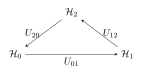
Operators on different tensor-product registers instead define many-body observables. Their product is not automatically transport on one fiber. The distinction must be fixed before designing a holonomy measurement.
Chapter 24 gives a corrected DG model of the actual infinite node, its clock lift and the endpoint-sensitive theta Ext calculation. A DG enhancement has and a graded Leibniz rule. A clock must commute with to act on cohomology. On , phases on the two terms can be chosen independently. On , compatible scalar actions agree but cohomology vanishes. Thus the differential alone creates no physical time. Higher operations have their own degrees and signs; periodic syzygies are not themselves a Hamiltonian or a time period.
A state-derived bifiltration can use increasing spatial radius and a decreasing correlation threshold. The order must give actual inclusions. For example, four edges around a square give an class; adding two triangles fills it. Multiparameter rank invariants, Betti tables and jump loci are meaningful diagnostics, but there is generally no canonical complete two-parameter barcode. Stability needs bounds on the actual filtration functions, including the statistical error of a nonlinear correlation-to-distance conversion. It does not identify a spectral or arithmetic determinant.
A renormalization channel needs an objective: which observables, states or phase labels should its coarse variables retain? Training selects parameters from data. This chapter supplies a solvable optimization task and a graph extension, while distinguishing an analytic optimum from an executed training run.
Entropy is , with . Reduced states use partial trace; mutual information is . We use natural logarithms. For
the reductions are , so and . The modular Hamiltonian is . At its flow is trivial although the pair is maximally entangled. Entanglement amount therefore does not determine a nontrivial local modular clock rate.
Proof. In a diagonal basis, the derivative under the trace is ; off-diagonal divided-difference terms have zero trace. Use . □
For the pair above, is exactly . The reference modular Hamiltonian stays fixed in this variation. A rank-deficient reference needs support control or a declared regularization such as .
Relative entropy is nonnegative, with equality only at equal states; incompatible supports give infinity. This is a strict matrix-convexity result, not the assertion that equality in a limit forces equality in an intermediate Hölder inequality. For the Gibbs state one obtains . A general reduced state has no automatically identified physical energy or physical time parameter.
On a finite graph assign symmetric regularized lengths
They define a shortest-path metric. Zero lengths would yield a pseudometric; infinite lengths could disconnect the graph. If two length assignments differ by at most on a graph with vertices, shortest simple paths have at most edges, hence their distances differ by at most . A patchwise bound can be smaller. The logarithm is ill conditioned near zero correlation, which makes the regularization and its error propagation part of the model.
A regular tree and are both hyperbolic metric spaces but have different boundaries, Cantor and circle, and are not quasi-isometric. Negative curvature does not alone give logarithmic diameter for every finite quotient. Expansion or a controlled family is needed. Arbitrary edge lengths need not form valid triangles for angle-defect curvature; metric-only curvature surrogates also require their neighborhood measures.
One can postulate a rate ratio for an entanglement proxy. This is a falsifiable ansatz. A bounded cyclic number expectation cannot increase forever, so an operational rate should use an unwrapped phase, counted transitions or calibrated oscillations. Matched noise-only controls must distinguish frequency changes from lost contrast. The entanglement-equilibrium route to Einstein equations has extra geometric, area, energy and continuum assumptions [126]. The finite first law does not supply them. Persistence can test stability across thresholds; it cannot convert this ansatz into Einstein dynamics.
A channel has Kraus form , . For unitary evolution followed by discarding one qudit,
The completeness identity follows by summing the environment projectors. An isometry would be injective and is impossible for . Stinespring instead adds an environment [127]. Outcome-dependent unitaries replace by . Ignoring the outcome remains linear; normalization of a selected branch by its success probability is nonlinear. Partial trace alone is not a nonlinear activation.
A solvable training objective. Encode inputs as , where , and choose
This encoding varies with its input; and do not. Anticommutation gives
The second term averages to zero for these real product states. Before training, this proves a limitation: that readout cannot retain . Richer objectives need a changed ansatz or another observable.
For targets , , put . The exact squared loss and gradient are
The minima satisfy and have zero loss. The stationary points must not be mistaken for a trained solution. A numerical optimizer can be tested against this answer; no run is asserted here. For comparison, CNOT followed by target- readout gives , a true two-input feature.
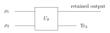
Give the graph its cyclic half-edge ordering and a proper edge-coloring. Shared two-site gates can run in parallel on each color class. A simple bounded-degree graph requires at most colors, not universally . Matching-based pooling specifies disjoint retained/discarded subsystems and a ribbon contraction. Independently applying channels to overlapping marginals does not automatically produce a consistent global coarse state.
Quantum convolutional and graph-network proposals offer concrete ansatz families [128, 129, 130]. A trained RG task may target phase classification, selected correlators, a reconstructed state, or an effective Hamiltonian. Success on one does not prove success on the others. A possible loss combines observable errors and symmetry penalties:
The penalty encourages cyclic weight sharing; exact equivariance requires intertwining by the architecture. Geodesic CNN coordinates and ribbon orderings are related design inputs, not identical constructions. Random quanvolutional circuits provide a useful untrained baseline. They must be compared with trained circuits and a classical model on the same data rather than credited with an automatic quantum advantage.
For a gate with , parameter-shift differentiation gives
Indeed the surrounding expectation has only constant, cosine and sine terms in this parameter. Other generators require a different rule. Finite-shot gradients and exact-state-vector gradients have different noise and optimization costs. Clifford layers can create entangled graph and GHZ states; non-Clifford gates are needed for universality, not for entanglement itself.
QGAT scores can be obtained from edge-register query/key circuits followed by classical softmax. For , is not Hermitian, so choose real quadratures
For example, gives real weights . The normalization is classical. The mixture is a state; a coherent sum of arbitrary unknown value states needs a separate physical protocol.
Generic amplitude loading of a -component classical vector can cost order input operations; qubits do not remove that cost. Several commuting heads can reuse one measurement basis, but their expectations still require repeated preparation. Quantum circuits are linear in ; nonlinear input encoding and classical processing are where these feature maps can become nonlinear in classical data.
A normalized readout uses positive effects summing to , with . An incomplete readout has sum at most and a failure effect. For orthogonal rank-one projectors and pure input,
This is exact. A common unitary preserves the templates’ inner products; it does not independently prescribe arbitrary nonorthogonal templates. Arbitrary projectors are not a POVM: two identical projectors give probability sum two at . A general Hermitian observable also need not be positive and cannot be interpreted as one rank-one pattern effect through a generalized square root.
For a two-pattern test, measure the computational basis on . Then and . A larger-probability rule retrieves zero for modulo . Sampling makes queries near the boundary difficult. This is a concrete retrieval task, not an exponential-capacity theorem.
Classical modern Hopfield networks have capacity and retrieval guarantees under specified separation, normalization and temperature assumptions [131]. Substituting for their associative dimension does not prove a QGAT memory theorem. A neighborhood with keys contains explicit candidates per head. Capacity requires a precision criterion, a dataset and a resource model. A -dimensional system perfectly distinguishes at most orthogonal states in one use; nonorthogonal packing, classical parameter storage and repeated queries are different resources.
Holographic reduced representations bind classical vectors by circular convolution. For the unnormalized discrete transform, . Correlation is an exact inverse only under additional nonvanishing/normalization conditions. A qudit’s determines diagonal populations when all modes are known, but no off-diagonal phases. Additional bases distinguish and , which have equal populations.
A channel hierarchy can be drawn as a tensor network with coarse bulk variables and fine boundary variables. Holographic-code models use a specified isometric encoding and reconstruction property [132]. Arbitrary discarding does not have it: a channel sending both and to one state destroys the label. A pooling tree alone proves neither boundary-area scaling of an actual state, error-correcting reconstruction nor AdS/CFT. These remain separate questions that a trained graph model can investigate.
An executable example must record graph, encoding, task, ansatz, loss, train/validation split, seed, optimizer and stopping rule. It should save parameters, predictions and loss history, compare classical and untrained baselines, and distinguish exact, finite-shot and hardware expectations. A noise study must name the channel and where it is applied. A successful finite toy task does not certify a thermodynamic RG limit, quantum speedup, Einstein dynamics or an arithmetic determinant.
The solvable pooling objective supplies a precise acceptance test for the separate executable examples. A training result is reported only when its checkpoint and verification outputs exist. The mathematical model and its analytic optimum remain meaningful independently of such a run.
An architecture needs controls, interactions, preparation, measurement and a noise model. A coupling graph supplies none of these calibrations by itself. Exact small operations provide useful acceptance tests before considering larger processors or molecular assemblies.
For a contraction , the map
is an isometry: its squared norm is . It extends to a unitary with an environment. Postselecting zero realizes with probability . Tracing out the ancilla includes both branches and does not produce just as a trace-preserving map. An operator of norm above one must first be scaled, with its success probability and amplitude normalization accounted for.
Amplitude damping has Kraus matrices
Direct multiplication gives and multiplies the excited population by . Pure dephasing instead can preserve populations while reducing coherences. Under a Markovian qubit model, ; these relaxation times alone do not determine pulse calibration, leakage or gate fidelity.
A Hadamard test estimates ; a changed ancilla basis estimates the imaginary part. Repeated preparations are required. Local randomized measurements and classical shadows can reuse settings for many observables, with locality-dependent costs [133]. Entropy is nonlinear, so a linear-observable sample bound does not automatically estimate mutual information. Reconstructing small marginals or using dedicated purity/entropy estimators is necessary.
At sites and maximum degree , at most edge marginals are needed. This defines a proposed workload, not an available processor specification. Routing, state preparation, correlated readout errors and reset must enter a resource estimate. Likewise qudits of dimension eight require at least binary qubits, before ancillas and coding. A generic encoded qudit entangler does not cost merely two-qubit gates. Its actual compilation and unused basis states must be checked. An infinite rotor needs a cutoff and a bound on leakage/aliasing; a cyclic quotient and a hard truncation have different boundary behavior.
Lanthanide-binding peptides offer chemically programmable spin organization. Rosaleny and collaborators reported ensemble pulsed X-band EPR in frozen solutions at 4 K, with representative relaxation values [134]:
| Complex | ||
| GdLBT | approximately s | approximately s |
| NdLBT | approximately s | approximately s |
Driven nutations motivate a molecular-spin platform, but are not randomized-benchmark gate fidelities or individual single-shot register readout. Proposed multispin organization and transport interfaces must be distinguished from a demonstrated controlled multi-qubit processor. Binding-affinity improvements are not measurements of increased coherence.
PDB 1TJB is a 2.00 Å Tb-bound structure [135]. Its motif has seventeen amino acids, YIDTNNDGWYEGDELLA, with a terminal amide entry in the deposited entity. Eight nearby oxygen donors come from Asp3, Asn5, Asp7, the Trp9 backbone carbonyl, and bidentate Glu11 and Glu14. Deposited residue identifiers and sequence indices need reconciliation in atomic constraints. Replacing the metal or scaffold requires new coordination and magnetic validation; a Tb structural model is not already a calibrated Gd or Nd control model.
An effective spin Hamiltonian is
Selecting a qubit requires a named transition, selection rules and leakage bounds. In a positive-field spin- Zeeman model, the lowest states have ; the central transition is not the lowest doublet. Spectroscopic selection can still use it, but must not be justified by a false energy ordering.
For an ideal two-level splitting , the thermal polarization is
At GHz, K; at 4 K the polarization is only about . Initialization near a pure state needs a separate protocol. A peptide’s melting temperature and a spin’s operational temperature therefore answer different questions.
Choose the laboratory drive convention
The resonant rotating-wave approximation gives with the stated rotating-frame convention. For , a pulse of length gives , equal to up to phase. A virtual changes the microwave reference phase; avoiding a separate physical pulse does not mean infinite fidelity of all subsequent gates. Spectral separation and drive strength control the approximation and leakage.
For dimensionless , isotropic exchange is , with in energy units. If swaps qubits, then , so
| (27.1) |
Thus gives SWAP up to phase and gives . The latter sends to a Bell-type superposition proportional to . It is not iSWAP: an XY Hamiltonian omits the term and has different evolution. Whether a peptide pair realizes any of these models needs measurement; dipolar anisotropy and -tensor orientation can be essential.
Echo decay, nutations, addressability, gate fidelity and single-shot measurement are distinct experimental tasks. EPR generally measures an ensemble signal. CISS and spin-dependent transport are possible future interfaces, requiring a calibrated relation to a qubit observable. A discussed SOMO–lanthanide exchange energy is not a measured Ln–Ln exchange across two nanometres. A fitted law also needs consistent units: with cm, Å and Å, it predicts about cm, not an order-one coupling. Geometry and chemistry must determine an actual model.
RFdiffusion3 supports atomically conditioned protein design and structural benchmarks [136]. Proteína-style backbone generation and BoltzDesign-style inverse-predictor optimization are complementary candidate methods. None guarantees a target spin coherence time, interaction graph or gate. A reproducible calculation pins a release, checkpoint, input schema, atomic identifiers and constraints; generated structures become preserved inputs for later evaluation. Current RFD3 documentation uses structured input specifications and its model-specific design interface, not an assumed legacy RFdiffusion invocation.
A conservative motif workflow fixes a resolved coordination cage, specifies metal/donor atoms and the intended state, generates surrounding scaffolds, assigns sequences with fixed motif positions, and tests structure and metal-aware energetics before synthesis. Hydrogen-bond conditioning is not a lanthanide coordination validator. RMSD and prediction confidence are filters, not physical yields or gate measurements. A small-motif benchmark does not guarantee a pass rate for a seven-motif, 1000-residue assembly.
ThermoGFN-IF can be formulated as a proposed multi-fidelity optimization [137]. SPURS supplies mutation stability predictions, BioEmu-v1 protein backbone ensembles, and UMA learned atomistic energies and forces in evaluated domains [138, 139, 140]. Model domains matter: BioEmu-v1 does not explicitly represent metal ions and their donor-oxygen geometry, so it cannot directly certify an intact Ln cage. All-atom reconstruction and a separately validated metal-aware calculation would be extra stages. Atom-count throughput is not a certificate of spin-vibronic accuracy.
For declared dimensionless scores define . If positive denotes destabilization, its stability reward contribution should have a negative sign. A GFlowNet aims to sample terminal candidates proportionally to this specified reward. Trajectory balance compares full forward/backward path probabilities to the terminal reward; subtrajectory balance additionally uses weighted subpath constraints. A unique construction path restricts the legal backward policy. These definitions can be implemented and tested without claiming a synthesized or operating processor.
Increasing melting temperature need not monotonically raise a Debye scale, suppress a particular spin-phonon channel or improve . At a fixed transition frequency, Bose occupation depends on that frequency and the temperature, not directly on bulk rigidity. A dephasing power law needs its spectral density, coupling operator and mechanism, including direct or Raman processes when relevant. One nanosecond of dynamics does not alone estimate a converged folded/unfolded partition-function ratio. Proposed tables mapping to numerical coherence, gate fidelity and fault tolerance are therefore hypotheses, not measured outcomes.
A regular tiling has sides per face and faces at a vertex. At curvature , a face has angle and area . In a closed genus- quotient, , and . For ,
| (27.2) |
Then as Gauss–Bonnet requires. The orientation-preserving triangle group has coarea ; a torsion-free subgroup has index . Its reflection triangle has half this area. The Klein quartic, with usual model , has genus three and . It is not a construction of every proposed quotient.
For a simple cubic tiling graph, its line graph places a qubit at each edge and joins pairs that share a vertex. Each qubit has four neighbors; the line graph has vertices and edges. Quotient degeneracies such as loops or repeated incidences need separate counting. Equal hyperbolic edge lengths do not automatically become equal Euclidean separations or physical couplings in an assembly.
A finite graph can be embedded and routed in three-dimensional space, but this does not create a complete smooth isometric in . A gyroid has varying intrinsic curvature. Schwarz–Pick concerns holomorphic metric contraction, not an SE(3) protein-placement algorithm. A finite assembly needs target Euclidean coordinates, distortion and steric bounds, mechanical constraints and explicit chemical ownership of shared sites. Kabsch alignment is a least-squares rigid fit; it does not remove inconsistent global distances. Two independently generated chunks cannot both contain one supposedly shared physical peptide without an actual chemical construction realizing that sharing.
Let a finite connected closed orientable cellulation have
This is a chain complex, not a short exact sequence. Its first homology is precisely the code’s logical information. Put qubits on edges and set , . A binary row defines an product and a row a product. Their commutation sign is , so the boundary identity proves commutation. The code is the common eigenspace in , not a binary kernel intersection regarded as that Hilbert space.
Proposition 27.1 (Surface-code dimension and distance). For this genus- cellulation,
Distance is the smaller weight of a nontrivial primal homology class and a nontrivial dual homology class.
Proof. Connectedness gives , and the one-dimensional top homology gives . Thus . A commuting error is a cycle; multiplication by stabilizers changes it by a boundary. A nontrivial logical is therefore a nonzero homology class. The dual argument treats errors. □
A noncontractible separating curve can be null homologous. Searching one geometric systole therefore does not certify a code’s distance. In a code, vertex checks have weight three and face checks weight seven; a global swap of conventions also swaps the logical descriptions.
At genus thirteen, (27.2) gives 504 data qubits and 26 logical qubits. If , the genus is 25 and . The asymptotic rate is . A cellulation gives and rate . Syndrome ancillas add physical resources. Suitable hyperbolic quotient families have logarithmic distance at constant rate [141, 142]; topology alone gives no such lower bound for every quotient, or distance eight for an unspecified finite surface. A finite certificate needs its incidence matrices and primal/dual logical-operator search. Logical qubit count grows linearly, not exponentially, with the number of physical qubits.
A finite acceptance test. An periodic square cellulation, , has , . Thus and : a straight winding row or column gives an -edge logical cycle in either lattice, and a lifted winding cycle must traverse at least edges. This yields with weight-four checks. The ranks verify directly. This is a useful exact decoder test before claiming a larger unprovided hyperbolic instance.
A storage code is not yet a fault-tolerant computer. Generic exchange and Zeeman terms do not commute with every stabilizer. An interaction meeting a check on exactly one site anticommutes with it, giving a commutator of order the coupling. Syndrome extraction needs ancillas, controlled operations, reset and measured error models; three exchange pulses alone do not prove nondemolition parity measurement. A threshold is conditional on code family, decoder and noise model. Code-capacity noise with ideal checks and circuit-level noisy checks are different. A gate estimate from another model cannot be compared to one threshold and declared fault tolerance.
A physical graph, a complex Belyi dessin and a rational arithmetic model are different data. A passport need not determine a Galois orbit, and one finite dessin cannot support a faithful action of the entire absolute Galois group on its finite sheet set. Frobenius requires descent and good reduction. Measured couplings do not automatically recover an Euler factor. The earlier finite-field theta benchmark is a concrete comparison test with its already specified scope, not a global GRH proof.
There is a useful circuit sanity check. XY exchange annihilates , so its exponential fixes it. A network of these gates, on an all-zero register preceded only by diagonal rotations, has a vacuum overlap that is just a phase. It cannot generate -function zeros. Also for Hermitian is not generally unitary at complex . Finite products are exponential polynomials in , not degree- polynomials; their unramified factor zeros have , not the critical line.
A Hilbert–Pólya proposal still has to identify its determinant with the same completed arithmetic function, including gamma and conductor factors. The transformation fixes a zero on the critical line; it does not reverse the ordinate. Conjugate twists matter for complex characters. Chiral symmetry is extra structure. An unbounded -paired self-adjoint spectrum has no Gibbs trace ; or is a different diagnostic. Similarly needs a spectral restriction away from negative shifted modes and a treatment of continuous spectrum.
These chapters give finite calculations, trainable channels and concrete experiments. They preserve the physical research program while leaving its arithmetic determinant, purity, convergence and positive-realization obligations explicit. They establish no complete proof of GRH.
Renormalization changes the description while preserving a specified set of physical predictions. To make that claim testable, we carry the effective action, its constant, observables and scale convention. Neural state compression and principal-axis alignment can be useful auxiliary techniques, but their training losses do not replace these objects.
A compression score does not specify an RG transformation. Following the real-space formulation of Wilson and Kogut [81], we specify the eliminated variables, effective action, normalization and scale map. Our exact finite decimation is distinct from an approximate tensor-network truncation such as Levin–Nave TRG [82].
Definition 28.1 (Finite classical RG step). Let the fine configuration be , with finite nonempty sets , and dimensionless log Boltzmann weight . Define
The full action includes its additive constant. A truncation or a learned approximation is a further operation with its own error, not this identity.
Proposition 28.2 (Partition, observables and composition). One has , and the normalized expectation of every observable depending only on agrees in the two descriptions. Eliminating and then equals eliminating at once, with the same tensor labels and inverse temperature.
Proof. Exponentiating the definition gives . Sum over , optionally multiplying by an observable , and divide both sides by the same strictly positive . Reordering finite sums proves the composition statement. No projection onto pair interactions is used. □
For an even homogeneous periodic Ising chain, write the transfer matrix as , . Its partition function is . Summing alternate spins replaces by and by ; the physical spacing doubles. Writing , its positive entries determine
These three parameters reproduce every entry of , so no normalization is lost. At , and the eigenvalue-ratio correlation length of the homogeneous extension in blocked units halves. Its product with the spacing stays fixed. The fixed points in are ; the latter is zero temperature, not a positive-temperature transition. Odd dessin examples below use the full-action definition, not this even-chain shortcut.
For odd , the clean dessin , has two black vertices, white vertices and one face; its genus is . Its incidence graph is with clean edges. Its infinite locally gentle order quiver instead has vertices and completed DVR-rank . We place physical spins on the incidence vertices; this is a specified finite spin model, not a faithful representation of that infinite algebra or order. The abstract incidence graph alone does not recover the ribbon embedding or genus.
With and fixed nonuniform fields , choose
Summing the two black spins gives the entire effective action
Every one of the physical edges is present, although its couplings belong to a tied three-parameter family. The Walsh expansion , with , is unique by Boolean orthogonality. It retains the constant and genuinely generated higher-body interactions. Our genus-two and genus-four examples use and continue by exact nested marginalization. Dropping all terms of degree greater than two is displayed as a measured approximation.
For a finite Hermitian Hamiltonian on nonzero finite-dimensional and , define
The matrix is strictly positive: for , sum the strictly positive quadratic forms of over an orthonormal basis of . Its Hermitian spectral logarithm is therefore defined. The identity proves partition and retained equal-time observable preservation by the partial-trace property. Repeated traces compose. The full Pauli expansion, including its identity coefficient, is retained. It is generally nonlocal and depends on ; this statement does not preserve all fine real-time dynamics or supply a local zero-temperature/thermodynamic RG fixed point.
FiniteRG.lean checks nine actual finite scalar marginal, exponential-action, partition, observable, composition, error-sandwich and transfer-trace statements. The quantum spectral-log and complete thermodynamic/field-theory interfaces are not formalized by these lemmas. These physics constructions give no arithmetic determinant comparison or new GRH conclusion.
This incidence schematic displays the physical elimination, not a planar uniformization of the genus-two surface. The explicit and face cycle determine the ribbon embedding; the interactive laboratory shows actual radial lifts and labels its four-real-coordinate projection.
Proposition 28.3 (Classical action-error propagation). If at every finite configuration, then . The partition ratio lies in . Every further exact marginalization preserves the same action bound.
Proof. The pointwise inequalities survive finite summation. Taking logarithms proves the first assertion; summing also over the retained variables proves the second. Iterate the same argument. For normalized measures the likelihood ratio lies between and , so a bounded observable error is at most . Per-step learned errors would add; a single initial error does not grow under subsequent exact elimination. This scalar proof is not an assertion that the matrix exponential is operator-monotone. □
The implementation checks full enumeration against the closed black-spin formula, Walsh reconstruction, raw partition equality, retained-spin magnetizations and two-stage versus direct elimination. At the quantum , limit, every Pauli coefficient agrees with the classical effective action, with the required minus sign between energy and logweight. At nonzero transverse field the model is
At general , the classical zero-transverse-field limit uses , including the fixed white fields, rather than scaling only the three varied controls. For , its full dimension is 128 and the first retained dimension is 32. Every one of the 1024 five-spin Pauli coefficients is computed; later retained dimensions are 8,4,2. Spectral-log/exponential and full Pauli reconstruction residuals, exact-trace composition and retained-observable comparisons are recorded separately. Floating-point residuals are numerical checks of the proved finite identities, not interval certificates.
The local laboratory exposes every scale, coupling/field controls for the classical model, selected generated interaction supports on actual dessin radial lifts, the even-chain trajectory and physical correlation length, and three fixed quantum matrix calculations. Live quantum parameter sliders are not offered for uncomputed Hamiltonians. Pair truncation carries the identity term and reports both partition and probability/density errors. A late-scale floating-point loss of the small eigenvalue is avoided by transporting the exact log-eigenratio coordinate ; this is explicitly the transfer RG identity, not a newly diagonalized value.
The learner targets all 32 unnormalized logweights of the spin decimation. Its three inputs are , with ranges . Fixed fields are . Seed 20261103 fixes 160 input samples, a 120/40 train/test split, and 40 OOD samples with , . The three feature qubits encode the couplings by . Two local layers, with a CZ triangle after each, contain 12 nominal optimizer angles. The final three phases commute with the measured products and are structurally inactive for this loss; they still change the displayed state phases. We count them as nominal parameters, not additional effective expressive directions. Seven nonempty Pauli- products feed an affine readout. There are 268 parameters. Feature registers are not the seven physical spin sites or five quiver vertices.
The training objective is full-action MSE, including the constant; KL alone would ignore that constant. A training-only ridge fit initializes the head, then 120 Adam updates optimize both circuit and head. Actual PennyLane analytic expectation calls implement the feature circuit. Parameter-shift derivatives of each feature are combined with the classical head gradient; full-loss finite differences agree to . All data, parameters, intermediate checkpoints and complete loss curves are preserved.
The held-out full-action MSE is approximately 0.00985, mean , mean TV 0.0290, and mean absolute log-partition error 0.0610. A classical quadratic-feature baseline with the same 256 readout parameters obtains 0.00613,0.00240,0.0233 and 0.0138, respectively. OOD action MSE increases to 0.267 for the quantum hybrid, versus 0.0555 for the baseline. The quantum-feature constant MAE is 0.0444 and higher-body coefficient RMSE is 0.00900, versus 0.0124 and 0.0130 for the classical baseline; different metrics favor different aspects. The aggregate results show no quantum advantage. They expose genuine full-action approximation errors rather than substituting state-compression success for RG.
Each saved example computes its maximum error over all 32 coarse states; the proposition then applies to its subsequent exact marginalizations. These per-example finite bounds are not uniform over the input parameter box. The synchronized architecture inspector shows literal gate outputs, Pauli features, head, logweights, generated interactions and partition value, linked to the exact genus-two dessin/order context. No full order representation, continuum universality, material-specific accuracy or arithmetic zero-location bridge is inferred.
A further executed node/edge-token hybrid uses the same exact RG teacher, with frozen three-qubit features, trained Q/K/V and a full-action head. Softmax, componentwise max-plus and hybrid variants are compared with a matched classical feature model; the latter has lower held-out action error. An explicit intervention-code/change variational MI objective learns concept directions; a 61-candidate latent forest and a held-out analogy transfer are scored on exact physical observables. Rips is actually reduced over , and a continuous Gaussian GFlowNet trains a trajectory-balance objective with specified root/Lebesgue measures. Empirical residuals do not prove exact terminal sampling, semantic reasoning or categorical equivalence.
The physical bit-flip repetition channel is separately executed and has under ideal recovery. A genuine cellular CSS calculation on the genus-two one-face dessin gives : vertex-incidence rank 6, zero face boundary, X-distance 1 and Z-distance 4. Thus this cellulation provides no useful protection merely from its genus. These finite layers, full formulas, proofs, parameters and scope are developed in the research book and interactive laboratories; the physical models are not faithful representations of the infinite completed order and supply no GRH bridge.
On the genuine dessin quiver write with indices modulo 5; cross-branch consecutive pairs are forbidden. Remove both arrows with source 0. The surviving algebra has vertices 0 through 4, arrows for , and relations for . It is an explicit finite gentle quotient, not the completed order itself.
Every surviving positive path stays on one branch and has length at most 4. For length there are paths, while length 0 contributes five idempotents. Therefore . The forbidden-chain resolution already proved for monomial gentle algebras has two alternating chains of length from vertex to when , and none for . Applying Hom to simples kills its arrow differentials. Hence and . The split finite-dimensional simple-module criterion gives .
Every full branch cycle crosses a removed arrow, so the common completed order parameter maps to zero. Thus is a finite -torsion quotient, not a DVR-free surface order. The difference is visible in derived Hom: is projective over , whereas in the original completed order the two forbidden arms of length 5 return to vertex 0 and give . The exact restriction along is consequently not derived fully faithful. This supplies a concrete cut on which to investigate graded gentle/Fukaya models, while proving why its equivalence cannot simply be transported to the original completed order. Boundary/stops/line-field data and an actual module-valued neural decoder would still have to be supplied. Exact path and endpoint enumeration accompanies the prose proof; this cut/category comparison is not claimed wholly Lean formalized.
The companion separates three objects: an exact combinatorial dessin, a chosen visualization of its surface, and a finite operator model. Agreement of their dimensions is not an equivalence of categories. We give constructions for which these distinctions can be checked directly.
For odd , let be the smooth compactification of
The affine curve is smooth: simultaneous vanishing of and would force , which does not lie on the curve in characteristic zero. Its double cover of the -line branches over the roots of unity and infinity. Riemann–Hurwitz gives .
Proposition 29.1 (Clean passports and infinite orders). The degree- Belyi map has passport
Its contracted dessin has two vertices, edges and one face. With darts , one may take
The associated completed order has -rank , and the polynomial locally gentle algebra is infinite dimensional.
Proof. Over zero, is a local coordinate at the two points , and has index . At a root of unity, is a local coordinate and , giving index two. At the unique point at infinity, has pole order two, so has pole order . Away from these points, differentiating introduces no further branching. This proves the passport and the Belyi property. The two cycles describe the two lifts of the radial segments in the -plane. The involution exchanges their lifts at the clean branch points. For odd , is a single -cycle: its square advances two steps in each -cycle, and two is invertible modulo . Hence . Each permitted -cycle repeats without meeting a forbidden pair. This proves infinite dimension; the earlier split-order theorem gives rank . □
For this gives genus two and order rank fifty; for genus three and rank ninety-eight. These are actual cellular dessins, not finite-dimensional stand-ins. The all-degree resolutions are obtained by iterating their forbidden successor permutation, as in the general resolution theorem. The number of vertices of the algebra is , while its coefficient-order rank is ; they should not be interchanged in a quantum register count.
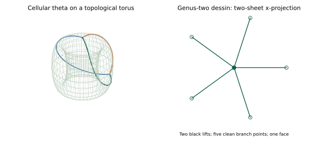
The same exact family gives genus five (, rank242), genus nine (, rank722) and genus sixteen (, rank2178). These ranks refer to the infinite completed orders over , not finite vector-space dimensions. The browser includes these examples and a four-dimensional rotation control: write in real coordinates , rotate the plane, then project to three coordinates. The omitted coordinate and projected intersections are explicitly identified. This is a view of the affine double-cover sheets, not a claimed injective embedding of a compact higher-genus surface.
A separate example is the infinite regular hyperbolic tiling. Its heptagons have angles , so the defect formula gives area at curvature . For a regular tiling, its central polygon’s Poincaré circumradius is
To derive this, bisect the polygon into right triangles with acute angles and . The hyperbolic right-triangle identity is , while the disk radius is . Substituting and applying elementary sum-to-product identities gives the formula. The condition ensures positive real radius.
A side is an arc of a circle with center and squared radius , orthogonal to the unit disk. Its endpoints determine and the analogous equation for . Circle inversion gives its hyperbolic reflection
If a side is a diameter, the circle formula is replaced by reflection in the line through the origin; the implementation handles that case separately. Reflecting adjacent polygons constructs finite windows of the infinite tiling. The implementation caps both depth and tile count and reports those bounds. It never calls a truncated window the whole infinite lattice. An optional Lorentz-hyperboloid view maps to , satisfying . Its metric is Lorentzian ambient data, not the Euclidean metric of the rendered mesh. A finite compact surface quotient, its side pairings and an arithmetic correspondence would require separate certificates. The current lattice patch supplies none of them.
The genus-one examples use a standard torus parameterization
The theta paths lift from to with translation vectors in the universal covering plane. Their interiors are disjoint on the quotient, and their complement is a disk; the induced rotations at the two black vertices give the one-face theta dessin. The elliptic square uses the two fundamental loops. These are topological realizations; the induced Euclidean torus metric is not asserted to be the constant-curvature or uniformizing metric of the algebraic curve.
For , the companion instead plots a three-real-coordinate projection of the two sheets of . Branch cuts, changes of sheet and the compact point at infinity remain part of the mathematical construction. Projected sheets can meet. No injective embedding or numerical uniformization follows from a screen image. The Sage source gives exact passports, quivers, forbidden pairs and determinant calculations. The installed sage launcher on this machine points to a missing application, so those Sage scripts are supplied but have not been executed in Sage in this milestone. Exact stdlib Python checks independently verify the displayed permutations, genus and ramification counts.
For , let , , with . Then
Applying the two sides to proves the first identity, including the wraparound because . The discrete Fourier matrix prepares the uniform superposition. The executable comparison applies , then , then , on a four-level carrier; its relative phases are nonconstant. Cirq, Qiskit and PennyLane statevectors are compared to the reference vector. Strawberry Fields realizes the same matrices on the single-photon subspace of four optical modes and compares the entire density block, including its off-diagonal phases. Preparing a Fock state need not leave the simulator’s internal representation marked pure, so reading only a ket would be incorrect.
The photonic cutoff two is exact for this passive, single-photon computation: photon number is preserved and no mode ever contains more than one photon. This justification does not extend to arbitrary squeezing or multiphoton simulations. Separate NVIDIA cuQuantum and CUDA-Q adapters and pinned upstream forks are provided. GPU execution is not performed on this Mac; source availability is distinct from a successful accelerator run.
These preserved experiments have distinct objectives. Local Ising regressors approximate selected coarse couplings but omit normalization and a full iterated action. QCNN compression, photonic principal-axis alignment and the Harper surrogate are auxiliary benchmarks. Actual partition-preserving RG and a trained full-action approximation are developed in Chapter 28. Here the exact targets, held-out samples, recorded seeds, classical optimizer and feature readouts are retained without calling these different objectives a complete RG flow.
For spins , summing the middle spin gives
where
Checking proves the identities. Thus the normalization and coupling have separate roles. The network below learns , not the full partition-function normalization .
For a three-valent star, let be boundary spins and sum its center. The exact boundary logarithmic weight is
Fourier expansion on the Boolean cube is orthogonal for . The symmetry removes every odd monomial. Consequently
This proves the zero-field star-to-triangle reduction and supplies exact labels. Such trivalent patches occur at the black vertices of the theta dessin. The associated Ising Hamiltonian is a finite model on that graph, not a faithful representation of its completed surface order.
The input patch is encoded by . Two layers of local rotations, a CZ entangler after each layer, and a final CNOT define an eight-parameter circuit . The three features are
A shared affine head predicts . Twelve trainable parameters include the four readout coefficients. Independent samples are drawn uniformly from : ninety are used for training and thirty are held out. The loss is the mean-square error against exact decimation. The independent constant predictor is fitted only on training targets.
For a gate , , and a fixed state and observable, the expectation has the form . Hence
Each gate parameter occurs once. The code differentiates the expectation features with this formula and then applies the classical chain rule to the squared loss and affine head. Applying parameter shift to the squared loss itself would generally give a wrong gradient. A central finite-difference check of the implemented full loss gradient is recorded.
The four-site periodic transverse-field Ising Hamiltonian is
We diagonalize its Hermitian matrix at thirty-six fields in , using the normalized lowest eigenvectors as input states. Every fourth field, starting at index zero, is held out. The circuit has two shared-layout local rotation layers with CZ edges on , followed by CNOTs and . Its sixteen parameters are optimized to minimize
The output on retained qubits is
Its Kraus maps are , so . Thus it is completely positive and trace preserving. For and any , each summand is nonnegative; cyclicity of the finite trace proves trace preservation. The Lean interface verifies the finite-matrix positivity and trace statements with explicit completeness hypotheses. It does not formalize the optimizer or claim convergence of an infinite renormalization flow.
The compression loss is the weight discarded by the chosen vacuum projection. Its successful decrease measures improved concentration for this finite input family. It does not imply exact recovery of arbitrary four-qubit states, an isometry from dimension sixteen to four, or a critical fixed-point construction. The held-out loss remains appreciable, and is reported without calling the model lossless.
The hyperelliptic dessin has genus four and completed-order rank162. Its nine edge labels index a permitted quiver cycle. A separate finite transverse-field Ising model is placed on this nine-cycle, with Hilbert-space dimension512. This uses the dessin’s combinatorics, without claiming a faithful representation of its infinite order.
The larger experiment uses twelve ground states over fields , with nine training and three held-out states. These are numerical lowest-eigenstate approximations. The residual alone is not a rigorous lowest-energy certificate. A sparse Hermitian eigensolver has maximum recorded eigenpair residual . The circuit has two layers of local gates and nearest-neighbor CZ around the cycle, with thirty-six parameters. Four CNOTs connect retained to discarded qubits, and tracing out four leaves a five-qubit output. Actual PennyLane gate simulation and parameter-shift gradients train for fifty updates. Final training and held-out discard losses are approximately and . These substantial residuals are reported: this architecture is not an accurate lossless coarse graining. It is a reproducible larger testbed, with saved parameters, held-out examples and numerical ground-state residuals. The local page permits comparison with the smaller four-qubit model, while retaining their different data families and capacities.
Three two-qubit patch encoders use the same eight circuit parameters on the three pairs of the Ising star. Let their features be . A learned query defines
There are eighteen trainable parameters. One hundred star couplings are sampled from , with seventy-five training and twenty-five held-out examples. The objective compares the three predictions with the exact Boolean-Fourier couplings above. The nonlinear attention head is differentiated by central differences of the complete training objective. This experiment is quantum-feature attention with a classical softmax head; it is not a fully coherent attention algorithm. The scalar labels do not assert permutation equivariance under conventions the implementation has not checked.

The Strawberry Fields experiment prepares two modes with opposite real squeezing and , then applies a fixed unknown-to-the-optimizer beam splitter angle . A learned shared beam splitter is optimized on twelve of sixteen squeezing values in , holding out every fourth value. With , the covariance convention is . The objective is
This follows by applying the real beam-splitter rotation to the diagonal covariance of the two squeezed modes. Since , its minimum occurs at modulo , with value . The code trains the angle with central-difference gradients and compares its result with this known optimum. Pooling subsequently discards a mode; the experiment itself optimizes principal axes before that discard. It is a Gaussian finite-mode surrogate, not a demonstration of an interacting field-theory RG flow.
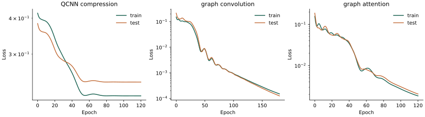
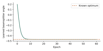
| Model | Initial held-out loss | Final held-out loss |
| Four-qubit QCNN compression | 0.38332 | 0.239725 |
| Shared quantum graph convolution | 0.213652 | 0.000125897 |
| Quantum-feature graph attention | 0.187065 | 0.00204477 |
The scripts in examples/quantum specify each circuit, data generator, random seed and optimizer. The approved isolated environment is recorded in requirements-cpu.lock; existing environments and all pinned Lean toolchains remain unchanged. NumPy reference and actual PennyLane runs are saved separately. Cross-framework tests exercise a nontrivial Fourier/clock/shift state, not just a vacuum on which every diagonal clock is invisible. The Strawberry Fields run uses its Gaussian backend for training and its Fock backend for the separate one-photon comparison.
The companion’s checkpoint slider selects a saved loss checkpoint. Its held-out examples use final weights; no intermediate predictions are implied. There are no hardware shots, cloud jobs or accelerator benchmarks. The training/test splits are deterministic interpolation tests on small synthetic families, not out-of-distribution or broad physical-validity tests. A model can help rank a proposed construction; it cannot discharge arithmetic holomorphy, determinant convergence, positivity or zero-location obligations merely by achieving low loss.
The trained models of Chapter 29 and the ToricGT references have a common computational interface: a finite directed acyclic graph whose vertices contain actual tensors and whose edges record the inputs to each operation. The local inspector at http://127.0.0.1:8765/architecture.html makes this graph navigable. Its scene is a computation graph, not a hardware layout or a physical embedding of the infinite surface order. The source code and numerical records are part of the project.
The twenty-two saved cases cover six trained CPU model families and six fixed-weight reference variants. The QCNN4 and QCNN9 weights, shared two-qubit convolution, quantum-feature attention, Gaussian photonic pooling and finite Harper hybrid are replayed without further optimizer steps. The classical TokenGT-style, tropical, block-ring, attention-hybrid and two expert-routing variants use explicit seeded weights. They are executable miniatures, not upstream trained language-model checkpoints. The adjustable forward clock is a separately computed finite carrier. GPU and hardware execution remain unavailable, and optional upstream heads remain proposals unless their own numerical evidence is supplied.
The record contains the source/checkpoint hashes, seed, conventions, formulas, shapes, axes, parameter values and checked errors. Each saved record is immutable and content addressed; its SHA-256 is verified before the interface accepts it. The inspector never changes the trained weights. Selecting a forward-operation step is not selecting a training epoch.
Two different attention mechanisms illustrate why the axes matter. The trained quantum-feature model produces three feature vectors,
Softmax here runs over three patches. The classical reference has seven token positions, including one padded node, model width six and two heads. After projection and splitting, its have shape . These heads are different from the three observables of the quantum circuit. Its also undergo the source’s maximum shift and Euclidean normalization before dot scores.
![PSTLrorooftacjmiaFeanl/icxePcxtedaoedo qtnd/ruct gnaheromn sxaratotpmxuf aha-mtmffilpantoilupxekzesaedthncceshohaenedatessdxst
Qα,pKFrX,:e[dV1[3i:,:]c:2,ti[1,7[3 co,[1,,n7,33: [,2]]36,[3]]7],3]](main14x.svg)
The shape labels are literal exported dimensions. The two columns are different finite models; no equivalence of their learned functions is asserted.
For tropical aggregation, a scalar output is
The inspector shows every maximizing key and the gap between the largest two legal values. A tie means equality of computed floating-point values, not a symbolic equality certificate. A query with no legal key has zero context by an explicit guard. Invalid block entries are stored as zero with a validity mask; including these zeros in a maximum would be incorrect. Softmax weights displayed in tropical records are comparison diagnostics rather than the tropical aggregation rule.
Soft-MoE dispatch normalizes across valid tokens for each expert-slot; combination normalizes across expert-slots for each valid token. These are different axes. Strict-prefix slots exclude the current and later token indices, while equal-rank attention can permit different tokens with the same reveal rank. The two rules must not be conflated into a stronger causality assertion. Likewise padding can acquire projection bias in a residual, so its mask must remain in later routing and pooling.
The stored StatePrep input precedes the displayed circuit. The variational gates have their exact wire order and angle metadata. Qubit zero is most significant. For QCNN9, the final CNOT targets start at wire five; the retained density matrix has shape , not a five-qubit pure state obtained by discarding amplitudes. The partial trace follows the unitary gates and is distinct from their dimension-preserving action.
The photonic model uses covariance order and . Its ellipse is a one-standard-deviation contour of a selected two-coordinate Gaussian marginal, with the marginal covariance taken from the actual intermediate record. It is not a plot of a trained interacting field theory. The Harper page separately displays the learned proposal and the fifteen exact rational principal-minor certificates. Rejected proposals are labelled as repaired. The carrier uses backward , so ; the live forward-clock example instead has .
The interaction reference is Brendan Bycroft’s LLM Visualization, reviewed at the pinned source revision recorded in planning/reference-inspector/source-manifest.json. Its model overview and self-attention walkthrough place the narrative beside dimensioned tensor planes, parallel query/key/value projections, attention heads and residual paths. The source’s picking code maps a selected output cell to input rows or columns and dot-product terms; its camera code interpolates toward walkthrough targets. These specific mechanisms motivate the local redesign. Reference hover inspection was limited by a renderer crash; source inspection is distinguished from successful live observation.
The local implementation uses original browser code and the project’s own immutable records. Its spatial scene follows dependency ranks and semantic lanes, rather than putting every operation in an identical card. A tensor’s dimensions determine its grid; head planes, selected literal coordinates and level-of-detail windows remain labelled. Overview retains the whole recorded computation, while a focused step moves toward its neighbourhood. The narrative gives the actual operation and evidence type. Supported cell expansions show numerical input terms and their computed result; other operations retain graph dependencies without inventing a scalar derivation. Surface and circuit views explain a separate geometric or physical interpretation of the finite carrier.
The rendering is a lightweight axonometric projection rather than a copy of the reference’s WebGL engine. Neither perspective effects nor a quantum-state array make an attention model a coherent quantum transformer. Checkpoint replay, fixed-weight reference calculations and separately proposed extensions keep their different status throughout the interface.
Choose an evidence category and example, then a step. Clicking an input follows its recorded dependency. Head/token/coordinate controls select literal array slices; paging exposes large states without pretending that a small viewport is the entire tensor. Color is a display convention and the selected coordinate gives its numerical real and imaginary parts. A zero amplitude has undefined phase and is labelled accordingly. Playback visits the forward pass, and stops when cases change or the tab becomes hidden. Orbit and zoom change the view, not the state or physical model.
The shared numerical records have independent quantum-backend and scalar reference checks. Browser checks exercise all saved cases, coordinate selection, masks, playback, view controls, circuits, covariance and certificate panels. These computational checks do not imply complete Lean formalization, generalization beyond the samples, quantum advantage or the arithmetic positive-determinant comparison. The general path/category and arithmetic interfaces remain the research obligations described in the final chapters.
The words “token” and “graph” have two different roles here. A TokenGT position represents a node or edge with features and incidence metadata. A tokenisation position instead represents a boundary in a word; an edge jumps across a contiguous substring. ConvexTok, introduced by Tempus, Whittington, Schmidt, Komm and Pimentel, Tokenisation via Convex Relaxations, arXiv:2605.22821v1, optimises the second representation. We derive its small finite formulation, reproduce its six-word example, and give new certified examples for finite arrow-word corpora of our infinite surface algebras. This supplies an auditable compression layer; it does not identify the two kinds of token or change a trained graph model.
Let be a finite multiset of nonempty words over a mandatory alphabet . For each word introduce boundary vertices . Include an edge for each allowed contiguous token . All single-symbol edges are free in the vocabulary budget, but cost one each in the segmentation objective. Longer candidates form a finite set . Equal strings have the same colour even when they occur in different words or positions. Candidates never cross word boundaries.
Write for occurrence flow and for selection of token type . Use incidence entries at an edge’s source and at its target. For each word let be at its initial boundary and at its final boundary. Separate unit-flow equations are equivalent to joining adjacent word terminals as in the paper: each word boundary must carry one unit, and there are no edges across words. The finite programme is
| (31.1) |
Requiring gives the integer problem. On the acyclic position graph its flow is one path per word, hence one segmentation. Conversely any segmentation with at most extra token types gives such an integer point. Consequently the LP optimum is a lower bound for the integer optimum . The constraint is per occurrence: selecting once permits both occurrences in , whose cost is two. Replacing these constraints by would incorrectly prohibit that reuse.
For a fixed discrete vocabulary , the exact segmenter is the backward recurrence
It returns a shortest path and a decoding by concatenation. Longest-first greedy need not do so: for and extra vocabulary it returns , whereas the optimum is . This segmentation issue is separate from BPE’s greedy construction of the vocabulary itself.
A floating solver’s proposed objective alone is insufficient for an exact lower-bound claim. Our original CPU checker writes the LP in the form
where and includes every upper-bound row . It uses SciPy/HiGHS from the already approved environment to propose primal and dual solutions, reconstructs rational entries, and then checks every condition with exact rational arithmetic:
These are executable rational witnesses, not a claim that floating-point optimisation itself is a proof assistant.
Proposition 31.1 (Finite rational certificate). Every feasible primal obeys for any dual pair satisfying the displayed inequalities. Equality with one feasible certifies the exact LP optimum.
Proof. Since , the componentwise dual inequality gives
The second inequality uses and . Equality therefore matches a lower and an upper bound. □
Independently, our checker exhausts every size- subset of and runs the shortest-path segmenter on each. This covers the at-most- problem, because adding candidate tokens cannot increase a shortest-path cost. For , all candidates suffice. Every stored witness is checked; deliberately perturbed primal and dual witnesses are rejected.
The paper’s Det rule chooses the largest ; Bias chooses the largest ; Int retains only values essentially equal to one. Our certificates are rational, so Int uses exact equality to one and Det/Bias use lexicographic tie-breaking. After choosing tokens we recompute a discrete shortest path; a fractional flow is not itself a tokenisation. An integral colour in one LP solution need not be present in every optimum. For example, with word and candidates , either single-token choice is optimal.
The paper’s example is
The mandatory-symbol count is fifteen. BPE first creates , saving three positions, then two merges save only one each: its cost is ten. Choosing instead gives nine. Our exact primal/dual pair has value nine, and all candidate vocabularies confirm . All three rounding rules give nine on the saved LP solution.
Our first new example is
One optimal fractional vocabulary has
with all other values zero. Its per-word costs are , totalling ten; the rational dual certifies optimality. The integer optimum is eleven, witnessed by vocabulary with costs and confirmed by all vocabularies. Det and Bias also yield eleven, while Int yields fifteen. The LP is therefore genuinely fractional even though its objective is an integer.
A second original corpus,
has . Its nonzero colour weights are and . The per-word fractional costs are . Exhausting vocabularies certifies the integer value. These examples demonstrate a relaxation gap; they do not supply a universal approximation ratio for rounding.
Set for , and retain the existing clean dessin of , . On put
There are two vertex cycles, edges and one face, so . Its polynomial algebra is the infinite locally gentle algebra
Here products are written in travel order: traverses first and then . A left-operator matrix convention reverses these products. Define the nonzero permitted word . Our finite multiset is
Each arrow label is one alphabet symbol, even when its printed label has several characters. The duplicate first word retains its multiplicity. We allow every occurring subpath of length two or three as an extra candidate. The LP bound consequently concerns this explicitly restricted candidate set, not arbitrary-length vocabularies.
| symbol count | subsets checked | ||||
| 2 | 5 | 20 | 29 | 19 | 190 |
| 4 | 9 | 36 | 41 | 31 | 630 |
The exact witnesses attain these values, and Det/Bias/Int all attain them on the saved LP solutions. A token names a finite permitted subpath; concatenation recovers every original arrow, hence its quiver endpoints and original path length. This is finite corpus compression, not a finite-dimensional quotient of . Arbitrary token concatenations may fail composability and need their own endpoint checks. Neither an algebra homomorphism on a freely generated token algebra nor a representation of arbitrary completed formal sums is asserted. The completed order still has rank over ; its rank, coefficients, multiplication, relations and modules are not reduced by counting tokens.
The companion laboratory at http://127.0.0.1:8765/convextok.html exposes the position DAG, literal fractional flows, vocabularies and discrete segmentations. Its five corpora and sixteen budget cases have sixteen exact primal/dual certificates and 2,312 exhausted integer vocabularies in total. The browser independently recomputes segmentation costs from local arrays; it does not solve a new LP when a user changes a vocabulary. The primary paper’s NLP training and large GPU experiments are not reproduced. Compression of a finite path corpus proves no module or Fukaya equivalence, arithmetic determinant comparison, or GRH statement.
This chapter connects executed finite methods through the same physical RG teacher. The completed order, ribbon dessin, physical Hamiltonian, token sequence and auxiliary quantum circuit retain their different dimensions. The surface is not reconstructed from a neural embedding, and the network is not silently declared a module over its completed order.
The genus-two clean dessin of Chapter 28 has five quiver vertices and DVR-rank 50. Its physical incidence model has seven spin nodes and ten incidence edges. Our TokenGT-style input has these 17 valid node/edge tokens and one masked padding position. Each token carries its type and endpoint metadata through an explicit three-angle encoding. The normalized auxiliary state uses data gates, fixed rotations, CNOT , CNOT and fixed rotations. The measured features are
These are three feature qubits per token, not the seven physical spin sites or a faithful representation of the infinite order. The quantum feature map is frozen; the Q/K/V matrices and nonlinear readout are trained. A separate literal replay of the pinned elliptic-theta fixture is retained with its own input hash and category boundary. The physical RG training input is the genus-two incidence graph, not that different theta fixture.
With , , and , define, on valid query/key indices,
Padding is masked in both softmax and max-plus operations and in pooling. The tropical output is a componentwise max-plus aggregation, with actual maximizing-key witnesses. It is not merely an argmax-key copy. A tanh context/residual pool and classical head predict all 32 coarse logweights, including the constant. These are quantum–classical transformers on measured features, not a coherent softmax unitary. TokenGT [83] motivates the node/edge organization; no general upstream expressivity or benchmark theorem is asserted for this compressed feature map. Numerical token-row permutation transport is checked, separately from arbitrary graph-relabel invariance and information lost by the encoding.
Four models use the same 120/40 split,40 OOD cases, seed 20261103, shared initialization/batches,900 Adam updates and 1,076 trained parameters each. The fourth uses six classical trigonometric features and the same hybrid head. The teacher is exactly from the seven-spin physical model, so partition, constant and retained-observable errors have physical meanings. The controlled input has three tied parameters, not 31 freely varied output couplings.
| Features/context | action RMSE | log RMSE | magnetization RMSE | mean TV |
| Quantum/softmax | .10261 | .09247 | .01773 | .03420 |
| Quantum/tropical | .06530 | .05923 | .01846 | .02167 |
| Quantum/hybrid | .10125 | .09653 | .02709 | .03212 |
| Classical/hybrid | .04878 | .04712 | .01565 | .01663 |
The classical baseline has lower held-out full-action error. Quantum OOD RMSE ranges from.555 to.763, versus.591 for the classical hybrid. One seeded experiment establishes neither quantum advantage nor general OOD robustness. The raw cases, every optimizer step and saved parameters are preserved. The tensor inspector replays actual token states, gates, Q/K/V, masks, scores, contexts and readout, and separately exposes the trained concept critic and continuous-GFlowNet MLP/density computations, with synchronized physical and algebraic support labels.
Let be a pooled embedding. We learn three normalized directions and a critic; their span need not be the whole embedding space. Choose uniformly among the six direction/sign codes and define
A fixed vector is not a random variable: the random objects here are the intervention code and its induced embedding change. The GraphCG-inspired [84] objective is cross entropy for predicting from , plus . For any normalized critic ,
Indeed the conditional cross entropy is conditional entropy plus an average nonnegative KL divergence. The held-out empirical functional is approximately 1.78844 nats. Its sampling estimate is not a certified lower confidence bound on an unknown population MI, nor proof of semantic identification: deliberately injected codes can already be distinguishable. The orthogonality penalty concerns the learned directions; it does not replace this probability model by ill-defined “MI between basis vectors.” A training-only ridge decoder maps steered embeddings back to physical couplings, whose effects are evaluated with the exact RG teacher.
The latent forest branches along both signs of each learned direction, keeps a width-three beam and searches depthfour. All 61 candidates are scored by exact coarse log and the five retained magnetizations. Its best saved reward changes from to ; the residual is substantial. This is finite branching optimization in embedding space, without a claim of human or general language-model reasoning.
A distinct analogy test estimates a mean displacement from transformed training pairs for , clipped to the training domain, and transfers it to 40 held-out embeddings. Decoded couplings go back through the exact physical teacher. Log RMSE is.09578 versus.15417 without transfer; magnetization RMSE is.02332 versus.04012. These are measured transformation-transfer results, not unrestricted “emergent analogical reasoning.”
For an explicit finite point cloud with chosen metric, the Rips filtration contains each simplex at the maximum distance between its vertices. The implementation reduces the full boundary matrices of vertices, edges and triangles over , with faces ordered before cofaces at ties. A zero reduced edge column creates a one-cycle; a later triangle pivot kills its class. Triangles suffice to compute . The 12-point learned embedding cloud has one positive-length interval approximately . The target and transferred physical-observable clouds, scaled as , both have empty positive-length barcodes and pair-distance RMSE.29095. Empty matching barcodes alone are not faithful analogy. The 67-radius independent checks test this finite calculation, not a physical topological-order invariant or a mirror theorem.
The executed GFlowNet [85] has root measure , three time steps, Lebesgue measure on each later chart and deterministic termination at step 3. The forward MLP gives normalized Gaussian means and learned diagonal variances. At the backward kernel is
the final backward transition to the singleton root has unit probability. The positive terminal reward is
The physical controls lie in a compact box, so the log-partition factor is bounded and the Gaussian confinement makes integrable.
For a path, the trajectory-balance residual is
If this identity vanished almost everywhere for every path, exponentiating and integrating the normalized backward kernels would give . This proves the desired terminal law under the exact density identity. A small empirical squared residual is not that identity and supplies no automatic global sampling guarantee.
Training uses 10,000 fixed continuous off-policy trajectories and 1,800 updates. Fresh held-out TB MSE is.002579 and on-policy MSE.002782. Learned log-normalization 1.70832 compares with finite-box quadrature 1.70734. Ten thousand new terminal samples give approximate histogram TV.04859 against a 20-by 20 midpoint histogram comparator on , with cell width.5. The separate log-normalizer quadrature uses a 201-by 201 grid with spacing.05. Both grids are verification, not the state space or policy. Tail/quadrature/sampling errors are not interval certified. The two-dimensional physical latent chart is not a full-support flow on all six pooled embedding coordinates.
For a logical qubit, use the repetition isometry , . Measure and , and apply the X correction specified by the two syndrome bits. Under independent X noise of probability on each physical qubit and ideal encoding/recovery, the weight-zero/one errors recover the state. Weight-two/three errors leave a logical X. Hence
The same channel identity holds with an entangled reference. The executed four-qubit Bell-reference density calculation compares actual BitFlip noise, syndrome projection and corrections with an independent eight-pattern sum. At its entanglement fidelity is.972, versus.9 without coding. It corrects one X error under the stated ideal assumptions, with no phase protection or universal fault-tolerance claim.
Applied independently to each auxiliary token-feature qubit, this is an explicit physical feature-memory layer. For a measured Z product of weight , the unencoded X channel multiplies its expectation by ; the recovered channel replaces by . This follows by conjugating Z by X and tensoring the single-qubit channel identity, even for entangled feature states. It distinguishes actual syndrome recovery from embedding regularization or persistence diagnostics. The resulting attention/readout is evaluated on all 40 held-out physical RG actions. At , hybrid full-action RMSE is.89766 without coding,.31589 after one ideal recovery level and.10608 after two, compared with clean.10125. Tropical RMSE changes from.32676 to.11810 and.06733, compared with clean.06530. Seventy-five explicit logical-X density-mixture comparisons on actual entangled token states agree with the attenuation rule within . The separately checksummed evaluation preserves every trained checkpoint. The three auxiliary feature qubits require 3,9 and 27 total physical qubits at zero, one and two recovery levels. The reported evaluations use the proved logical-channel identity, not a full noisy 9/27-qubit gate simulation; encoding and recovery gates are ideal throughout. Concatenating ideal blocks gives the noise recursion , improving ; it is not an RG theorem about the physical Hamiltonian.
Proposition 32.1 (The one-face dessin is not a useful quantum memory). The CSS construction with qubits on the 10 clean edges of the genus-two dessin, vertex X checks and its single face Z check has parameters , with X-distance 1 and Z-distance 4.
Proof. The connected graph incidence matrix over has rank . Every edge occurs twice in its single face boundary, so the face boundary is zero. The chain relation holds. For independent commuting Pauli checks that do not generate , the projector is . Only its identity term has nonzero trace, so its rank is . Thus the CSS logical dimension is . All single-edge X operators commute with the zero face check. No singleton edge set is a cut/coboundary, since each edge lies on a four-cycle; thus it is not an X stabilizer, and the X-distance is 1. A Z logical operator is a nonzero cycle because the face-boundary subspace is zero. The simple bipartite graph has girth 4, proving Z-distance 4. Exact enumeration independently checks the ranks, commuting checks and shortest logical witnesses. □
Genus and logical dimension therefore do not imply noise protection. Useful surface-code families require controlled cellulations, local checks, growing primal and dual systoles, a stated noise model and verified decoders.
For real numbers and ,
Factor out the maximum; the remaining sum lies between 1 and . This is a precise zero-temperature max-plus limit. Replacing the finite-temperature RG sum by a maximum discards entropy, including its normalization. An attention semiring alone supplies neither the physical energy calibration nor the valuations and curve/disk counts needed for tropical geometry and mirror symmetry [86].
For a categorical connection, Section 28.2.4 gives an actual 25-dimensional finite gentle cut with global dimension 4, kills , and proves that restriction to the original completed order is not derived fully faithful. It is a constructive starting point, with a proved obstruction to transporting comparisons indiscriminately. Choose its grading and verify the relevant homological smoothness before invoking a geometric model. The partially wrapped Fukaya comparison for smooth graded gentle algebras requires boundary, stops and a line field [66]; it is not a blanket statement for the complete order on the original closed surface. One could then compute specified Hom/Ext or arc-intersection data and use them in a categorical learning objective. No such equivalence or learned categorical functor is produced by the three-qubit feature circuit. Physical RG marginalization is not automatically a derived equivalence either.
For materials models, one must supply a physical Hamiltonian/data family, symmetries, locality constraints and validated observables. The executed finite spin problem is a reproducible statistical-mechanics testbed, not a materials-discovery result. An executed five-qubit generative example uses a saved learned coarse action to compute and prepares . Born probabilities reproduce to . This coherent pure state is not the mixed Gibbs state. Applying the explicit local projector-Kraus dephasing channel gives with the same residual. From 4096 seeded quantum Born samples, the maximum five-magnetization sampling error is.04377; the simultaneous 95% Hoeffding radius is.05086. The union bound uses for five observables in . This bound controls shot error relative to the learned distribution, separately from its physical teacher bias. All 32 amplitudes are computed classically, with no efficient many-body preparation or quantum advantage claim. Sampling latent coupling controls, predicting a full action and generating physical configurations is therefore a concrete finite hybrid route, with its costs and errors exposed. Quantum-information uses of the physical feature-memory code require the stated noise/recovery model. None of these numerical, categorical or physical interfaces establishes the missing arithmetic Frobenius/determinant comparison for GRH.
All optimizer histories, source hashes, parameters, held-out/OOD data, barcodes, candidate rewards and density checks are preserved. The six-panel laboratory and four trained architecture passes display literal arrays and gate states; the original 22 architecture records remain unchanged. Exact finite CSS enumeration and the bit-flip channel proof are distinguished from floating-point learned diagnostics. The finite classical RG identities are kernel checked in FiniteRG.lean; general neural optimization, continuous GFlowNet sampling, quantum recovery and categorical interfaces are not thereby wholly Lean formalized.
This chapter connects explicit learned functions to physical RG targets, categorical path calculations and checked quantum circuits. Each width, coefficient field and category is specified before comparisons are made.
Learned functions enter this program as candidate generators, physical surrogates and control laws. A network may suggest an arithmetic metric, operator or gluing datum; a successful fit does not establish its positivity, analytic domain or identification with a completed -function. Those are independent mathematical obligations. This section gives explicit interfaces and executed examples rather than treating “quantum”, “tropical” or “infinite width” as a substitute for that comparison.
Proposition 33.1 (A specified quantum-feature width limit). Let , and be independent, and set . For independent features,
almost surely on every specified finite set of pairs. Every is a positive semidefinite Gram kernel. For a readout with only trained, its tangent kernel is exactly . These statements do not assert the same limit for a jointly trained finite quantum transformer.
Proof. Uniform-phase integration gives . The Gaussian characteristic function then gives . Products are bounded by two, so the strong law applies to each pair and hence any finite union. For any finite coefficient vector , the Gram quadratic form is . Differentiating with respect to gives the final assertion. □
The frozen-kernel squared-loss flow has residual when the loss normalization is absorbed into time. Null directions do not decay. A complex feature space instead uses the Hermitian kernel . A finite coefficient field has neither this Gaussian law nor an ordered positive Hilbert metric; changing algebraic coefficients is a separate operation.
Proposition 33.2 (Tropical limit and a cancellation boundary). For real and ,
An attention maximum therefore has a controlled log-sum-exp approximation. It does not by itself define a tropicalization of a variety or an HMS functor. In a valued coefficient field, valuation of a sum can increase by cancellation.
Proof. After subtracting , the exponential sum lies between one and . For the second statement, both and have valuation zero in , whereas their sum has valuation one. In characteristic two that sum is zero. Thus replacing every addition by its tropical minimum without tracking leading coefficients loses information. □
Kontsevich–Soibelman constructions require valued analytic and integral-affine gluing data; appropriate gentle/Fukaya comparisons require specified categories, gradings, stops and smoothness hypotheses [92, 91, 93]. Learned coefficients can propose such data, but the compatibility equations and arithmetic comparison still need proofs.
Executed physical examples. On the actual clean genus-two dessin, put seven quantum spins on its incidence graph and compute a normalized Gibbs state. Exact white-spin partial trace gives a two-spin quantum RG marginal. Twelve RTX4090 runs train four-qubit-feature diffusion and flow-matching models for its smoothed -measurement law: two objectives, entangled/product circuit controls, and three seeds. They have 5,810 nominal parameters and 2,000 steps each. A separate four-qubit variational purification flow learns the full known density interpolation, with 48 controls. Its minimum fidelity on a 33-point grid is ; this is not a uniform theorem or universal noise inverse. The matched controls show no consistent entanglement advantage.
Actual cuStateVec/cuTensorNet execution also covers 7-, 11- and 23-qubit finite circuits on genus-two, genus-four and genus-ten dessin incidence graphs. The 23-qubit case has 8,388,608 amplitudes and 447 gates. These larger circuits are untrained; the small cases have independent NumPy comparisons, while the largest has normalization and inverse-circuit checks. The exact environment and all failed/preliminary records are preserved.
Geometric and hardware interfaces. For the contracted -edge dessin, the graph fundamental group is , and its universal graph cover is the -regular tree. The theta case has a three-regular cover, distinct from the four-regular Cayley graph of . Neither is the coefficient field or the universal cover of the filled compact surface. Explicit path modules over the infinite genus-two algebra give Hom, Ext and Tor computations; Frobenius pants tensors give exact TQFT gluing, with a heralded physical implementation. CHSH gives a finite game benchmark, distinct from the unrestricted correlation separation in MIP*RE [99]. Three executable tropical hardware references and a source-pinned chip-design survey complement the circuits. They are arithmetic/control designs, not synthesized chips, validated CFT/string dualities or a proof of GRH.
Take , . Its clean incidence graph has two black vertices and five white vertices, hence seven physical spin sites and ten incidence edges. These differ from the five quiver vertices and the infinite-dimensional polynomial algebra. The physical Hilbert space below is finite; no faithful action of that whole algebra on it is assumed.
Let be Pauli matrices on physical site , with the black sites numbered zero and one and the white sites . Our executed Hamiltonian is
Here . All coefficients are dimensionless and inverse temperature is one. Diagonalizing the actual Hermitian matrix gives . We retain the two black spins:
This is an actual coarse quantum state, with trace one and positive spectrum. An independent Pauli–Kronecker NumPy reconstruction agrees with the saved matrix to . Its minimum eigenvalue is approximately , and its off-diagonal Frobenius norm is . There is therefore quantum coherence that a probability histogram alone cannot describe. No chemical or experimental material dataset is involved: this is an exactly specified finite quantum-matter benchmark.
Let for . The hybrid samplers learn
This is a continuous dequantization of the measured spin law. A sign measurement of these samples differs from by at most in total variation, by a coordinatewise sign-flip coupling and the union bound. This is below here. It is small compared with finite-sampling error, but it is not zero. The samplers do not recover phases or the entire . For example, and have the same diagonal but different density matrices.
For use the cosine cumulative noise schedule, with endpoint offset , clipped step variances between and . Write and . The forward noising law is
A network minimizes the ordinary mean squared noise-prediction error. It is a classical stochastic sampler containing quantum-circuit features, not an implemented coherent quantum channel. The executed reverse update uses
The last step is deterministic. Even an exact conditional noise predictor does not make this Gaussian reverse kernel the exact reverse mixture at finite : posterior uncertainty of the mixture component remains. The oracle-noise control therefore retains a reverse-kernel approximation, finite schedule and Monte Carlo error, not just a numerical integration error.
There is also an exact, known-teacher reverse-mixture control. Conditional on center , put and . At a supplied , draw the center with posterior weights proportional to . Then draw
These formulas follow by conditioning a jointly Gaussian pair with covariance . Starting from the exact forward terminal mixture and composing these reverse conditionals recovers exactly in distribution, up to numerical and sampling error. It uses the full teacher, so it is a diagnostic rather than a learned solution.
Independently sample and , set , and train toward . This is the conditional flow-matching regression objective. Conditional on center , its time- mean and variance are
Let be the corresponding mixture posterior. The exact conditional velocity is
Indeed ; Gaussian conditioning gives the displayed formula. The positive variance includes both endpoints. The code verifies this formula and the diffusion-score formula by independent finite differences of a separately written mixture log density. Learned sampling uses 128 Heun steps. Oracle-velocity sampling isolates finite integration and sampling error for this known smooth density; it is not an upstream QFM reproduction [94].
The neural input is . An affine encoder maps its seven channels to four angles through . A two-layer four-qubit circuit uses angle-reuploading gates and, for the entangled architecture, a CNOT ring. Fifteen commuting -string expectations are concatenated with the seven input channels. A SiLU head predicts noise or velocity. The product control uses the same nominal parameters and removes the entanglers. Final diagonal phase rotations are invisible to the all- readout; equality of nominal parameter counts does not establish equality of effective Fisher capacity.
Every run has 5,810 nominal parameters, batch size 512 and 2,000 Adam steps. There are 16,384 training draws and 4,096 disjoint held-out draws, with seeds 20261104, 20261105 and 20261106. The four architectures/objectives were rerun at every seed. The following figures are mean and sample standard deviation across those three runs, not confidence intervals or asymptotic theorems.
| Objective | circuit | sign-law TV | sliced |
| Diffusion | product | ||
| Diffusion | entangled | ||
| Flow | product | ||
| Flow | entangled |
The second metric uses sixteen fixed projection directions and an independent teacher draw. The experiment demonstrates learning but no consistent quantum or entanglement advantage; the product control has lower mean error on both reported metrics. No physical quantum processor, shot noise, industrial chemical prediction, OOD material transfer or complexity speedup was tested. All checkpoints, seeds, histories, runtimes and teacher controls are retained.
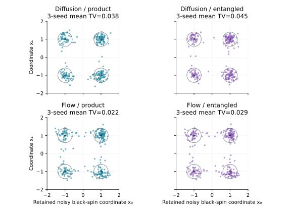
We separately implement quantum evolution, without identifying it with the classical samplers. Exact depolarizing diffusion is
It preserves trace and positivity and satisfies by direct substitution. Its linear inverse on all matrices is not positive: has a negative eigenvalue on the orthogonal complement of any rank-one projection when . Thus a learned inverse cannot be a universal deterministic physical channel.
For a constructive state-preparation benchmark, take the family , , and its canonical purification in . It is normalized because . The initial purification is two Bell pairs. We train a six-block four-qubit circuit: each block conjugates local rotations by a fixed CNOT network and its inverse; angles are . All blocks are identity at the control time zero. The 48 learned controls are trained against full known purification states, using the fidelity loss. This ideal supervision is stronger than access to measured samples and is accounted for explicitly.
An RTX4090 run of 2,000 steps, batch 64, gives minimum fidelity on a 33-point grid and maximum reduced-density Frobenius error . The reduced state is obtained by an actual ancilla partial trace and passes trace/positivity checks. These are grid diagnostics, not a uniform or out-of-family guarantee. The construction is a learned coherent control path for known targets, not a universally learned inverse to depolarization. Its full 76-gate replay and intermediate complex states are exported to the same numerical architecture inspector as the other models.
Proposition 33.1 fixes which width is being increased: the number of independent one-qubit features, with only their readout trained. At initialization let be independent standard centered readout coefficients, independent of the frozen features. Conditional finite-dimensional outputs are then exactly centered Gaussian with covariance . The almost-sure kernel convergence implies convergence of these finite-dimensional characteristic functions to the Gaussian law with covariance . This proves the specified finite-dimensional GP limit. It does not prove tightness in a function-space norm, parameter-feature learning, a many-qubit limit or a continuum QFT. For frozen , squared-loss gradient flow gives , whose eigencomponents decay at their kernel eigenvalues. A zero eigenvalue leaves a nonzero residual unchanged.
The executable width experiment fits the existing exact 32-configuration classical black-spin-decimated action on genus two, including its constant. This is a second true RG teacher, distinct from the quantum white-spin partial trace above. With 96 parameter triples for training, 32 for testing, eight feature seeds and ridge , widths 16 and 4,096 give mean relative kernel errors and and mean full-action test MSE and . The limiting RBF readout is also evaluated. Finite numerical convergence supports the implementation; the proposition supplies the limit proof. Quantum NTK literature requires its own parameterization, ensemble and lazy/large-width hypotheses [91, 90].
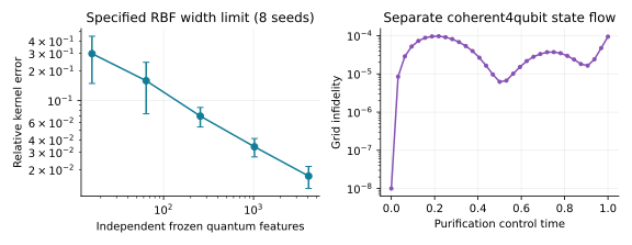
For complex embeddings the Hermitian Gram form, realification , and conjugation must be respected. An arbitrary real network on twice as many channels need not be complex linear. In characteristic two, ; an embedding into real vectors cannot be a unital field homomorphism preserving that addition. Finite-field path algebras and cellular/CSS computations are still meaningful, but Gaussian integration, ordered Gibbs weights and real backpropagation do not transfer by renaming the field. An explicit discrete learner over , , uses features and coefficients searched in the finite field to learn . All inputs are verified; an affine-only learner has nonzero minimum error. The trained map compiles to the permutation unitary on a complex Hilbert space of dimension . Retaining makes its inverse subtraction explicit. This is reversible encoding of a field-valued polynomial learner, not a field embedding into complex amplitudes or backpropagation in . Its training is exact finite coefficient search. A tropical semiring is not a field; coefficient cancellation, valuation signs and the underlying valued algebra must be specified.
For GRH, each architecture offers an experimentally testable role: quantum features can parameterize candidate metrics or probe observables; graph tokens can encode actual local incidence, masks and monodromy; tropical attention can search extremal valuations or active constraints; flow/diffusion can propose continuous operator/control parameters; RG can organize a genuine hierarchy of coarse actions. None of these roles proves that its Gram matrix is the arithmetic positive metric. One must still construct the arithmetic object with correct conductor, gamma factors, zero divisor and domain, prove compact-uniform control and zero location, and keep Dirichlet, Hecke, Dedekind and Artin hypotheses separate. A learned candidate is accepted only after its exact defining equations and analytic estimates are supplied.
Write , and for the free group, coefficient field and profinite completion, respectively. For a theta graph with vertices and edges , an explicit cover has vertices , , and edges
Left multiplication is the deck action. Contracting all -edges produces the usual four-regular Cayley tree of ; before contraction the graph is three-regular. Equivalently, vertices are reduced nonbacktracking edge paths from , with an immediately reversed edge cancelled. This gives a tree and unique path lifting in every length. Its radius- patch has vertices, hence 766 at radius eight. With a planar ribbon structure the abstract graph is a spine of a topological pair of pants. The actual dessin instead has the ribbon structure of a once-punctured torus. Forgetting the cyclic orders identifies the abstract graphs, not these thickenings. Graph distance is not automatically hyperbolic geodesic length.
For the contracted clean -edge dessin there are two vertices and parallel edges, so is and the analogous universal tree is -regular. The new examples include , of genus two and four. Reinserting clean white bivalent vertices subdivides its edges. Attaching the face to recover the compact surface introduces a relation; the closed genus-two surface has its surface group and a disk universal cover, not one of these graph trees. Separately, has fundamental group . The unbranched cover induced by a clean dessin removes all preimages of those three values. For our degree- map there are punctures; its Euler characteristic is , not that of the dessin’s one-skeleton. Thus the occurrences of in monodromy, graph covers and arithmetic profinite theory must not be silently identified.
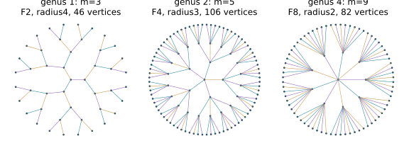
For finite-supported representations of a suitably graded bound quiver, pushdown maps split into deck-homogeneous blocks. The arrow equations preserve the degree, and monomial zero relations are homogeneous. The resulting Hom direct sum controls all deck pieces, not just degree one. For an explicit graph-only diagnostic two lifted edge intervals have upstairs endomorphism dimension two, but downstairs endomorphism dimension four: the deck pieces have dimensions . This graph-quiver calculation is not substituted for a dessin-algebra module example. The actual infinite polynomial module examples below supply that part. A Hom-controlled functor needs its specified exceptional/source/target subcategory and control statement; exactness, a deck-sum formula or equal dimensions alone is not an equivalence or an AR universality theorem. A derived comparison must control all and composition, together with an actual derived/enhanced functor.
To fix conventions, let be the earlier rightmost-arrow-first polynomial matrix algebra acting on left columns. Here we use travel-order path multiplication and write for the prose-identified bound-quiver algebra. Right representations therefore encode the earlier covariant left-column representations. There are vertices and arrows , with
Both pure branch paths survive at every length. No arrow-truncated finite algebra is being used. We work with ordinary polynomial modules, not with all completed lattices or all infinite strings.
Put and let be its residue simple. The augmentation kernel is . Multiplication by an arrow kills exactly the opposite-branch positive paths at its target, while each surviving path has a distinct normal image. Its kernel is therefore the right ideal generated by its unique forbidden successor, without cancellation. Iteration yields a projective resolution with
The two arms are indexed by alternating-branch relation words. The differential entry is the last arrow, not the product of the zero relation word. This kernel description proves exactness in every degree. Applying Hom to a simple kills every arrow entry, hence
Tensoring with the left residue simple gives the same Tor dimensions. A graded version needs its internal degree shifts. In particular the residue simples have infinite projective dimension in this ambient algebra.
Let be the one-arrow string supported at vertices zero and four, with and every other arrow zero. Its presentation is
The two images have disjoint normal-path support and span the kernel, because retains exactly . The next entries are on the first arm and on the second; continue by their unique forbidden successors. This gives an unbounded exact resolution by the same normal-path argument. Full arrow-commuting equations give
In the Hom complex for both adjacent differentials vanish, so . A concrete nonsplit self-extension has at zero and four, , , all other arrows zero. The first-coordinate submodule and quotient are . A section at vertex zero would lift the quotient basis to a vector with second coordinate one; sends it to a nonzero first-coordinate vector, contradicting commutation with the zero action on . Thus is not rigid in this actual ambient category. No almost-split universality is inferred from this nonsplitting.
For finite-dimensional let . On each finite idempotent projective the evaluation pairing identifies with . Dualization is exact on these finite-dimensional terms, so the resulting complexes give for the stated finitely generated resolutions. In particular . The exact program checks six source/target pairs through degree twelve, all five simple-target formulas and 250 normal-kernel samples. The unbounded resolution assertions rest on the normal-form proof, not on the finite cutoff. These new homological proofs are prose/exact calculations; full corresponding resolution objects are not yet Lean packaged.
A geometric path may label a string after specifying the ribbon structure, relations and category. Turning it into a geodesic needs a metric and appropriate boundary/stop data. Intersections compute morphisms only under the hypotheses of an actual graded/Fukaya comparison. The homologically smooth graded-gentle perfect-category theorems do not identify our entire ordinary or completed module category with the Fukaya category by inspection [93]. In particular the residue resolutions warn against silently imposing smoothness or finite projective dimension.
For , take , . In the ordered bases and , multiplication and comultiplication are
The pairing is , with determinant . Associativity follows from ; coassociativity sends one to the three placements of a single one among two ’s and sends to . On the four tensor basis vectors, all three maps in
give, respectively, , , , and zero. This proves the Frobenius identity. The unit and counit identities follow directly on the same basis. These are exact oriented 2D TQFT gluing data [95], not a presumed positive Hilbert structure.
The handle map sends and . Closed genus- contractions are . The genus-two value really vanishes in this example. In characteristic two the torus value also vanishes, illustrating a meaningful coefficient change rather than an embedding-space relabelling. After extending to with the Euclidean metric, and ; is not an isometry. The exact code constructs and a failure block with . Stacking them gives an isometry into , extendable to a unitary with ancillas. Its success probabilities on the four basis states are . Postselection implements with state-dependent success; normalizing the selected outcome is not the original linear map .
For a closed genus- surface a pants decomposition has pieces and sewn curves. Conformal sewing adds moduli-dependent propagators and analytic consistency [96]; string amplitudes need worldsheet, ghost and integration data beyond this finite tensor. A pants network or a hyperbolic graph is likewise not an AdS/CFT duality or a Ryu–Takayanagi derivation [97]. Such interpretations remain specified research targets until their extra structure is constructed. Arithmetic/anabelian reconstruction additionally requires arithmetic profinite fundamental-group data and its Galois structure under the proper field/curve hypotheses. Neither a discrete graph nor a coefficient module supplies that arithmetic extension [98].
For uniform input bits , CHSH accepts outputs when . With observables its success probability is , where
For a deterministic classical assignment one bracket vanishes and the other is , giving success at most ; all sixteen assignments are checked. On , take , . Then gives success . For arbitrary self-adjoint involutions, and each commutator has norm at most two. Hence , proving optimality. The exact matrix checker verifies the entire spectrum , not just a numerical sample.
MIP*RE, in its pinned v4, gives an external unrestricted correlation separation and a negative answer to Connes embedding [99]. We do not rerun its external formalization or claim a new proof of it. CHSH has its optimum on two qubits and the same commuting optimum by the preceding bound; it does not exhibit the general separation. A learned game strategy is useful for finite witness search and checked bounds, but unrestricted computability and dimension quantifiers cannot be settled by a finite game simulation.
The chip-design campaign pins twenty public repositories, twenty-four focused document ranges and thirteen primary papers. It covers AlphaChip/Circuit Training, independent macro-placement benchmarks, OpenROAD-family flows, quantum layout and low-level control. The source ledger records what was actually read, not a full audit or reproduction of every model. An exact public identity for the phrase “bare-metal Qiskit” was not established; no repository was invented.
Three original executable references implement a masked signed max-plus tile, an ordered mixed MAC/max-plus scheduler and a fail-closed synthetic IQ steering controller. Wide addition precedes winner selection and final saturation; earliest-index tie handling is explicit. Empty masks remain invalid, not an extra candidate of value zero. The controller requires a current calibration epoch, enough samples and a valid margin/deadline before allowlisting a steering action. Checks include all 65,536 signed eight-bit additions, 262,144 masked two-lane cases, reordered completions and twelve negative controls. These are digital reference models, not synthesized RTL, routed chips, measured RF feedback, power/area estimates or universal hardware speedups. A tropical context block can avoid multiplications inside that primitive while its projections, scores and other layers still require their own arithmetic.
The Linux snapshot preserves the Mac project, source clones, histories, checkpoints and environment archives. Linux GPU execution uses the existing Torch CUDA environment and a separately approved isolated cuQuantum prefix; macOS binaries are not treated as a Linux installation. The conda lock, setup instructions, gate/head replay records and all failures are retained. The on-page book contains one canonical laboratory for this chapter and links all five new checkpoint architectures into the existing tensor inspector. New physics, width and homological results have their explicit prose/numerical/external status; selected earlier Lean components do not constitute a full formalization of this extension or a proof of GRH.
A useful learned contribution must distinguish approximation of known -functions from proof of their zero locations. We propose holomorphic coefficient/readout learning, certified contour losses, arithmetic trace and functional-equation residuals, Schatten-controlled operator refinement, certificate search for the original signed moment, and exact-algebra representation constraints. Each has a different acceptance test.
For an analytic target on , let there and choose . A degree- holomorphic readout trained on equally spaced points of the radius- circle has the explicit uniform error budget
The following proofs give all four terms, a primitive-Dirichlet arithmetic bound for , and an infinite-feature kernel limit with its actual rates. Thus known analytic families can be approximated to arbitrary requested accuracy with independently certified evaluation error. This does not prove GRH. Uniform approximation by an already-real-zero determinant class is a different, potentially GRH-equivalent requirement; it must not be assumed through an alleged universal-approximation theorem.
The output is a complex holomorphic function, not an unconstrained real MLP on . Fix a center and a finite family of targets analytic on a neighborhood of the closed radius- disk. Certified values of and of an evaluation error are inputs to the quantitative theorem. They must be obtained without GRH or the desired arithmetic positivity. A finite conductor family uses the maximum of its independently bounded constants; this is not a uniform theorem over all conductors. Arithmetic character data are exact discrete inputs, not rounded embedding labels.
For primitive nonprincipal Dirichlet characters, the completed function is entire and a direct bound is given below. Pole-cleared zeta/Dedekind targets and known holomorphic Hecke or elliptic targets require their own explicit normalization and growth bounds. General Artin holomorphy is not assumed. Approximating on a compact domain avoiding possible poles does not prove that those poles are absent. Real/complex analytic norms, finite-field algebra and tropical semirings must likewise retain their distinct meanings.
Write and choose , integers and sample angles . Let , including all quadrature and rounding errors. The model and empirical objective are
This is a fixed holomorphic feature layer and a learned complex linear readout. It is a genuine convex learning problem; no nonlinear feature-learning claim is attached to its guarantee.
Proposition 33.3 (Four-part uniform error bound). Put , and . Let , and take gradient descent with . After steps from , on ,
The terms are optimization, certified sample error, Cauchy aliasing and analytic truncation, respectively.
Proof. Discrete Fourier orthogonality gives for , since . In real and imaginary coordinates the gradient is ; hence . Cauchy–Schwarz bounds its evaluation by , giving the first term. The displayed iteration is in exact arithmetic. A numerical FFT/GD implementation must also bound coefficient-rounding error; a coefficient error of norm adds at most to the evaluation budget. This is convergence to the projected least-squares optimum; the empirical residual need not vanish when the labels have components outside the model.
For exact samples, the Fourier coefficient divided by is . Uniform convergence on the sampling circle permits interchanging sums. Cauchy’s estimate bounds the alias by . Sample errors contribute at most . Multiply by , sum the two finite geometric series and add . These are exactly the last three terms. □
Choose , then , then and the optimization tolerance so that each displayed term is at most . All four can tend to zero; thus any fixed compact subdisk and finite independently bounded target family have arbitrary-accuracy approximation. This claim needs a certified oracle bound, not an empirical test-set MSE. The present high-precision demonstrator is explicitly numerical and does not relabel its floating evaluations as interval certificates.
Choose and use features . Their kernel has the compact-uniform limit
The geometric tail proves this limit directly; positivity follows because each quadratic form is a sum of squared feature combinations. The readout space is the sequence space with bounded evaluation on . On the radius- circle its population coefficient Gram operator is diagonal with eigenvalues .
Proposition 33.4 (Infinite-feature readout convergence). Suppose the initial coefficient error is in , as for zero initialization and the analytic target above. Population gradient flow has and converges in , hence uniformly on every . If and , then
For zero initialization this source condition holds whenever , with .
Proof. The diagonal loss gives the scalar ODE in each coordinate. Dominated convergence, with majorant , proves norm convergence. Evaluation is bounded by the geometric-series factor. Under the source condition, ; the maximum occurs at . Cauchy’s coefficient estimate gives , and summing the resulting geometric series proves the explicit source bound. □
There is no width-uniform exponential rate: . At finite degree the slowest mode has rate . Fourier whitening recovers the identity Gram matrix in Proposition 33.3, but its unbounded infinite-dimensional preconditioner must not be called a free uniform rate. Ridge adds a positive rate floor and a calculable bias; its coefficient bias factor is , and must tend to zero for unbiased convergence. A standard Gaussian-process initialization need not lie in the kernel’s RKHS; the stated hypothesis cannot be silently applied to it. These exact fixed-feature statements are distinct from the nonlinear NTK limits of deep networks [110] and from the trained few-qubit feature-learning circuits.
For a primitive nonprincipal character of conductor , parity and root number , put and . The standard primitive theta transformation and Mellin identity give
The character conjugation and root number are retained. These standard functional/analytic inputs are unconditional in the stated Dirichlet scope [111]; this text does not claim a new Lean proof of Poisson summation. Exponential decay makes both integrals entire in .
For , choose an integer and define
Integration by parts gives . Consequently is a valid finite upper bound. For a computable finite version, choose and sum through ; the remaining one-integral sum is at most
Indeed , decreases, and . Twice this tail covers both Mellin terms. The same bound controls theta truncation, with no assumption about zeros.
After truncating the sum and the integral, elementary interval exponential, logarithm, sine and cosine evaluation on a compact interval, with a bounded-derivative quadrature remainder, gives an arbitrary requested certified . The explicit exponential tails control both truncations. This proves computability of the oracle; it does not assert that an ordinary high-precision special-function call is already a validated implementation. For a finite conductor cutoff, take the maximum of the computed bounds.
Augment the coefficient objective with independent interval enclosures of on contours, derivative-weighted losses and adaptive samples near small . If on a Jordan contour, Rouché’s theorem transfers the exact interior zero count of to . An interval root count and a strict margin are acceptance conditions. Sampling finitely many heights alone proves no exhaustion of the off-critical domain.
Use exact character masks, conductor dependence, primitive Euler factors, gamma normalization and the conjugate functional equation as structural features or independently verified residuals. On , with , for the logarithmic-derivative Dirichlet tail has the elementary bound , from and integral comparison. This is a useful certified training region; it does not extend absolute convergence into the critical strip. A functional equation alone also does not locate zeros.
Learn compatible finite compressions, graph-norm/domain residuals, self-adjoint boundary conditions and uniform Schatten-tail bounds from the actual infinite dessin/order construction. Trace-norm convergence transfers ordinary Fredholm determinants, with the standard bound
[112]. Strong resolvent convergence alone does not supply this bound. A reciprocal critical-spectrum model typically needs a genus-one regularized determinant and Hilbert–Schmidt control; it must not silently be treated as trace class. The arithmetic determinant identification remains an independent obligation even when the learned operators are Hermitian.
For the actual original-family low-gcd moment, use adversarial legal masks, conductors, short rows and retained II–I covariance to search for a sharp envelope or counterexample. Rational/interval or exact symbolic checking must certify a proposed inequality uniformly. A sum-of-squares or dual certificate can prove its stated parameter box; extrapolating it to all conductors needs a separate analytic argument. Preserve exact locally gentle relations, surface-order completions, determinant semi-invariant weights and module category labels in the representation architecture. Small relation loss is not an exact functor or an arithmetic comparison.
Quantum feature Gram positivity is not Weil/arithmetic positivity. A proved finite Gram lower bound gives a readout rate, while growing width requires the actual limiting kernel and initialization hypotheses. Proof-guided co-training can learn proposed identities or compression maps, then export rational/algebraic candidates for independent Lean/interval validation. Validation, rather than a confidence score, decides which claims survive.
Proposition 33.5. No sequence of real-rooted polynomials converges locally uniformly on to . Every such polynomial has error at least somewhere on .
Proof. On that circle, . A smaller uniform error would, by Rouché, force a zero of the polynomial inside the disk, whereas all of its zeros are real and the disk misses the real axis. The same argument excludes local-uniform convergence. □
Thus a claim that an everywhere-real-zero/self-adjoint determinant family universally approximates the completed arithmetic target may already contain the missing GRH bridge. Hurwitz transfers zero-freeness only after independent local-uniform convergence and a nonzero limit have been proved. The analytic learner above deliberately proves approximation without asserting that spectral restriction. Its learned functions are evidence-bearing candidates, not a completed GRH proof. All new analytic/probabilistic statements here are prose proofs and scoped computations; no complete new Lean layer is claimed.
The next implementation step certifies growth and analytic-tail constants, while leaving sample evaluation and coefficient rounding separate. Put and, for an integer , define
The binomial coefficients give , so . Every evaluation of at a positive rational argument is exact rational. With the same as above, choose and let
This rational number bounds on the specified disk. Indeed decreasing to increases the positive integral majorant. For , the maximum of is . Split the Gaussian exponent into two halves, use , and sum the resulting geometric tail. Replacing its numerator and ratio by increases the bound, since its denominator stays strictly positive. This proves the formula.
For the actual conductors , center , radius , and , exact fraction arithmetic gives respectively , , . Using (or these integer upper bounds) and the rational radii , makes the Cauchy-alias and Taylor terms exact rational certificates as well. Full numerator/denominator records and the executable certify_learning_constants.py are supplied. This certifies constants, not the complex sample oracle, floating optimizer or GRH.
A two-player nonlocal game samples questions and scores outputs . The players may share a state, but communicate neither questions nor outcomes during play. Our finite tensor strategies have . Offline joint optimization is allowed and is distinct from communication during the game. We train local measurement frames and a Schmidt angle using the exact Born objective, and replay actual checkpoints, probabilities, correlations, word moments and simulated shots in the interactive laboratory.
For use the tilted score
Its classical maximum is ; its quantum maximum is [113]. At the uniform CHSH winning probability is . This conversion does not apply unchanged to the tilted objective. The three seeds for each of give nine trained runs. One run remains at the classical value ; the other runs reach the stated quantum maxima numerically. This retained failure rules out a claim of universal convergence of the optimizer.
The magic-square task uses two Bell pairs, local four-dimensional joint measurements, row parity and column parities . Its classical value is and its quantum value is , as proved below. Three further trained local-frame runs reach values within of one. All twelve runs are small CPU simulations with saved seeds and parameters, not hardware Bell experiments or evidence for quantum training advantage.
These examples belong to both the closure of finite tensor correlations and the commuting-operator set . The external theorem separates these sets and implies the negative answer to Connes embedding [115]. We do not reproduce that theorem. Finite learned strategies, positive state Gram matrices and finite NPA constraints do not witness its separation.
For deterministic signs, either or , so the CHSH term is at most ; choosing gives the tilted classical maximum . Convex mixtures cannot improve a linear objective. For self-adjoint involutions, with operators of different parties commuting, write . The exact identity
proves the CHSH quantum bound by positivity. Expanding the squares uses only the involution and cross-party commutation relations.
For the tilted case take , , and . Then . Choosing
with and , gives by direct substitution (including the endpoints). This verifies attainment; the universal tilted upper bound uses the sum-of-squares theorem in [113] for ; the endpoint follows by continuity since . This is not an unproved inference from our restricted two-qubit parametrization.
On two local qubits arrange the observables
Entries commute within each row and column. Pauli multiplication gives row products and column products . Alice measures a row, Bob the transpose of a column, and they share . The identity gives correlation one at every intersection. The product identities force the required parities. Thus they win every question pair and the quantum value is one.
A classical perfect table would have total product by multiplying the rows and by multiplying the columns, a contradiction. At least one of the nine question pairs fails for any deterministic assignment. Conversely, Alice can output all ; Bob outputs all in the first two columns and in the last, failing only one cell. The uniform classical value is exactly ; shared randomness cannot improve it. Our learner conjugates Alice’s observables by one local unitary and Bob’s transposed observables by , preserving each party’s parity and commutation constraints at every optimization step. The exact score is .
Finite strategies and noisy experimental laws. Unitary parametrization preserves valid projective measurements, so negative Born loss searches inside the chosen finite strategy class. Mixing the state with with visibility preserves positivity, normalization and no-signalling. For joint outcomes, ideal independent samples and , Hoeffding plus a union bound gives maximum frequency error at most with probability at least . Browser sampling is an illustration of this conditional IID statement. With dimension fixed, compactness and explicit matrix-product Lipschitz bounds permit exhaustive finite nets for arbitrary-accuracy global value approximation. Local gradient descent alone has no such guarantee.
Moment and dual-certificate learning. For words in measurement generators, define (or its mixed-state trace). For every , ; the mixed case follows by convexity. We compute these actual finite word Gram matrices, not an optimized outer relaxation. NPA learning may propose PSD moment matrices obeying word relations, while an independently checked identity proves an upper bound. A small residual is not an exact certificate. Successive NPA levels converge to the commuting-operator value under the hierarchy’s hypotheses [114]. Each level defines an outer relaxation; a validated optimized value or a dual-feasible certificate yields an upper bound. One feasible primal moment matrix alone does not bound the optimum and is not a realization theorem.
Tracial moments and Connes embedding. General vector-state moments need not be cyclic. A microstate learner for a tracial algebra must additionally preserve cyclic identities, positivity, norm bounds and compatibility across increasing word lengths, and compare with normalized matrix traces. Our displayed state moments do not fulfill that separate task merely because they are PSD. The external undecidability result [115] also precludes a single computable dimension/error schedule deciding all promised nonlocal games. It neither forbids certified solutions of specified finite games nor establishes any impossibility result for GRH. The valid connection to our program is certificate search with exact relation checks; neither Bell violation nor kernel positivity gives the missing arithmetic determinant/zero-location bridge. These new game proofs and computations are not claimed as complete Lean4 formalization.
The hubs-and-spokes construction in the HoTT book, Sections 6.6–6.8 [109], gives a useful language for attaching cells. For a loop , form the homotopy pushout : add a fresh hub and paths from every to that hub, continuously indexed by . This attaches a disk, rather than merely a finite graph of radial edges. The book’s Remark 6.7.1 explains why identifying the hub with an existing boundary point requires extra coherence; Remark 6.7.2 distinguishes propositional from judgmental computation.
For our dessins the useful distinction is geometric. A vertex star has a disk neighborhood with a specified cyclic ordering of its incident bands. Removing the disk center gives a punctured disk, which retains its peripheral loop. Removing only the vertex of a finite star instead leaves disconnected open rays. These operations cannot be interchanged. In a cellular dessin, filling a face imposes its attaching-word relation; leaving its center punctured retains a boundary component of the ribbon neighborhood.
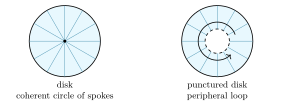
The shaded regions are two-dimensional; the displayed finite spokes sample them. The annulus shown on the right is a deformation retract of the punctured disk, not a missing vertex in a one-dimensional graph.
Proposition 33.6 (Face filling changes the covering problem). Let a connected cellular dessin be a spine of an oriented genus- ribbon surface with boundary components. Its graph fundamental group is free of rank . Capping all boundary components gives the presentation
For the one-face clean dessins and used here, these free ranks are respectively and , before capping.
Proof. A spanning-tree collapse of the connected spine leaves circles. The ribbon surface retracts onto that spine and has Euler characteristic , proving the rank formula. Cutting a surface along a standard system of handle arcs gives the boundary word . Van Kampen therefore presents its group by these generators and this one relation. With a boundary present, eliminate , leaving the stated free group. Capping attaches disks along the , so van Kampen sets each , giving the closed-surface presentation. For our rotations on , both black vertices have the same cyclic order on the incident edges. Suppressing the bivalent white vertices gives dart rotations and involution . The face permutation is one -cycle for odd . Thus , , , and , giving both examples. □
The once-punctured torus and closed torus both have , but their groups are and ; only the closed torus has . The analogous genus-two groups are and the four-generator surface group, with in both cases. Indeed the standard closed-surface cellular complex has one vertex, edges and one face. The face word is a product of commutators, so its abelianized boundary is zero. Removing the face leaves the wedge of circles. This computes the stated homology and also explains why alone misses the face relation. The torus group is abelian while is not; in higher genus the closed surface has nonzero while the graph does not.
Consequently the graph’s universal cover is a tree, whereas the universal cover of the filled genus-two surface includes lifted faces and is a disk. Collapsing a spanning tree changes the combinatorial cover graph; the Cayley tree of a free basis is not literally the original biregular dessin cover. This distinction matters when lifting strings, periodic paths and boundary conditions in the infinite locally gentle algebra.
The gluing language organizes local patches and their compatibility maps. It does not reconstruct the ribbon cyclic order, complex structure, Belyi map, quadratic zero relations, coefficient ring or polynomial/formal/operator completion from the homotopy type alone. These data are retained explicitly in the existing dessin and order constructions. Descent of modules, derived categories, Hom-control, AR meshes or Fukaya categories needs a separately defined functor and hypotheses; a homotopy pushout of underlying spaces is not such a theorem. Nor does it imply an arithmetic determinant identity.
The accompanying tool computes the same one-face genus-one/two/four dart families and draws local disk/annulus patches and their surface polygon presentations, peripheral loops and face words. These are exact finite combinatorial checks plus the topological proof above. HoTT is referenced as a conceptual foundation; no univalence or higher inductive-type axiom is added to the pinned Lean4 development. Its complete cell-attachment and categorical formalization remains an explicit task.
The learned program now has two additional, separately constructed corpora: 16,384 effective-material response records and22,951 molecular conformer/force records in their default configurations. Time samples are not counted as independent systems. Source-linked and dynamical configurations are additional. The active HolonForge/Aster and Mora-3 repositories were read only; no data, vocabulary, checkpoint, source enrollment or training process was changed.
The material corpus covers SSH, Kitaev, QWZ, Rice–Mele, Harper and actual clean-dessin classical RG models. The molecular corpus includes designed amides and peptides, with explicit-H MMFF94 calculations, geometric persistence, and method-labelled conformations. Forty-eight existing Aster MP20 structures, 32 existing Mora PubChem identities and eight public PDB structures supply separately labelled anchors. Their new computed responses are not new experimental observations, DFT labels, binding affinities or CISS measurements.
All conformer, gauge, intervention and task descendants share a partition. Specified physical/chemical similarity edges are closed transitively before component-level stratification. Large components are kept intact even when 80/10/10 proportions or rare-class coverage become impossible. This gives a finite, threshold-relative separation statement; it cannot guarantee every kind of statistical independence or prevent overfitting. Source anchors are train only. Molecular anchors are also checked against every default heldout using the same chemical and applicable geometric thresholds; conflicting parent groups are excluded. Global exposure to the models’ previous corpora is a separate evaluation gate.
For a number-conserving one-particle Hamiltonian , write and . The data use , occupations and outgoing currents . Then , directly from . Paired BdG evolution includes its independently computed condensate source; it is not falsely treated as electron-number-conserving normal transport. An exact interacting Hubbard dimer supplements Gaussian exchange correlations. Molecular nuclear dynamics uses MMFF94, with a separately labelled, uncalibrated effective -orbital model for charge modulation.
Parquet configurations retain condition, target and evaluation roles, source versions/hashes, units, failures and audit evidence. The local dataset explorer shows actual structures, currents, time evolution, graph wavelets and checked circuit compilations. These computations support candidate discovery and model validation; the independent arithmetic determinant/zero-location bridge remains open. No new whole-chapter Lean formalization is asserted.
Each default Parquet row has a persistent record identity, parent/similarity group, partition, evidence class, lossless scientific payload and typed numeric columns. Forward inputs have the prefix condition_; supervision uses target_; evaluation_ fields are excluded from inputs. The full payload, source hash, record identifier and audit text are not automatically fed into a model. Otherwise an apparent condition/target mask could still leak the target through metadata or a duplicated representation. An inverse task needs an explicit desired-condition contract and role change.
The origin fields distinguish a new simulation from a reused planned-source identity or geometry with new labels. The source-anchor configuration preserves existing train assignments. New public PDB coordinates retain their own source identity rather than being called members of PDBbind or newly acquired experimental quantum measurements. All anchors are train only: they do not establish blind performance on a model that may have encountered the parent.
The actual native interfaces are tested without changing either model. Aster accepts condition-only Hamiltonian records through its existing tokenizer. Changing a hidden target leaves those input tokens unchanged. Mora-3’s scalar graphs preserve computed/predicted evidence. Its existing scalar/array supervision interfaces reject those targets under their observed-only policy. That rejection is recorded, not bypassed by changing the evidence label. Source construction is therefore distinct from the owning model’s future admission, scaling, objective and evaluation decisions.
The two-band QWZ model uses
Its continuum band gap is . To see this, put , . The squared positive energy is , a bilinear function on ; its minimum occurs at a corner. Thus an odd mesh that misses cannot certify a gap near or2. The corrected release uses this analytic guard, even32/64 meshes, random gauge checks and an unavailable label near closure. The occupied-band integer uses the oriented link-product convention of Fukui–Hatsugai–Suzuki [100]; the sign convention is retained in the row.
For the Rice–Mele pump, take , and . With positive , minimization over first gives at ; minimization over gives the exact gap . Harper’s direct gap has a conservative mesh/Lipschitz guard, explicitly distinguished from interval certification. The displayed bulk slice has ; an open strip is evaluated separately at . A single strip is not a proof of its entire edge dispersion.
The SSH winding, Kitaev sign invariant and classical dessin RG retain their own hypotheses. Surface genus is not an electronic phase index. In the Kitaev row, a physical onsite defect changes particle and hole diagonals with opposite signs. Its gauge change has the form . These preserve the recorded particle–hole symmetry; arbitrary independent diagonal perturbations would not. A quarantined draft revealed this error before release. No failed draft replaces a verified artifact.
The molecular set contains explicit chemical graphs, atom order, hydrogens, stereochemistry, method-labelled optimized references and bounded coordinate perturbations. MMFF94 supplies empirical molecular-mechanics energies, analytic forces and partial charges [101]. It supplies neither ab-initio electron density nor experimental affinity, ADMET, redox or biological efficacy. An optimization convergence code is not a theorem of a unique global minimum. Absolute MMFF energies are not cross-molecule atomization energies.
The checker reconstructs the stored bond graph in its actual atom order. A canonical SMILES string determines chemical identity but need not give the coordinate-array order. Geometry-assigned stereochemistry is checked against that identity; mirror controls fail. Energies and forces are recalculated on every accepted record. Central energy differences check force signs/units, and proper rotations/translations check the expected scalar/vector behavior. Missing or unsupported labels are not imputed.
For the heavy-atom point cloud, the complete finite Vietoris–Rips2-skeleton gives over . All edges and triangles, including ties, are ordered explicitly. Independent boundary-rank calculations verify selected Betti numbers against the barcodes. These are geometric distance-filtration features; a molecular loop or persistence bar is not an electronic topological phase. MMFF and the idealized -orbital Hamiltonian retain separate labels.
Let be the finite parent set and connect two parents whenever a declared similarity test passes. Add edges for all shared source/variant lineages. Assign a partition to each connected component and inherit it for every row. If an accepted similarity edge joined two partitions, its endpoints would lie in one component with two assignments, a contradiction. This proves the exact finite no-crossing property for the declared relation.
For materials, normalized parameter and relative finite-spectrum thresholds are family/size-specific. SSH hopping swaps, Kitaev chemical-potential sign and the classical RG global-sign symmetry are folded conservatively. For molecules, stereo-agnostic constitution, nonempty Murcko scaffold and radius-two Morgan Tanimoto threshold form chemical components. A second all-conformer pass adds edges for equal heavy-element multisets with sorted pair-distance RMS at most Å. This descriptor is rotation/permutation invariant but is not a complete congruence invariant or a certified RMSD optimizer; conservative false-positive grouping is possible.
Whole-component allocation balances row counts and declared family/topology or molecular-size/persistence strata. It never breaks a component to manufacture an80/10/10 result. The large peptide component makes the molecular training partition much larger than80%; rare/held-out peptide coverage can consequently be absent. Exact distributions and cross-partition nearest witnesses accompany the release. Protein TM-score, homology separation and global overlap with the models’ complete historical corpora are not certified by small-molecule fingerprints. Threshold separation cannot itself guarantee freedom from all leakage or overfitting.
For normal free fermions, preserves Hermiticity, trace and the spectrum: follows by adjoints, trace follows by cyclicity, and is a similarity. Thus and projector occupancy remain valid. Computing the diagonal of gives
The currents therefore obey site continuity and conserve total particle number. Their arrows represent probability/particle flux, not measured trajectories of individual electrons. Charge modulation is in the declared electron-charge convention.
For a paired model, put and . From an initial Slater projector use . Evolve with the full BdG Hamiltonian and recover , . The independently computed pairing source is
The commutator derivative and this separate source formula agree in the checks; the source is not defined as the residual of the desired equation. For a Gaussian state, Wick’s rule gives, for , ; on the diagonal it is . The negative term is an exchange hole, not a computed Coulomb exchange-energy functional. Explicit small Fock-space evolution independently checks the covariance, current and pairing conventions.
The interacting control is the two-site Hubbard model at two electrons:
In its singlet/doubly-occupied symmetric sector the matrix is ; the triplet energy is zero. Diagonalizing gives the exact exchange gap , approaching for large positive . The full six-state two-electron sector supplies density, spin-swap and current trajectories; a separate16-state Jordan–Wigner calculation checks them. This finite dimer is not a thermodynamic phase classification.
For nuclei, velocity Verlet uses actual MMFF forces and masses, with explicit time/energy units, finite energy drift and momentum checks. A Grad-only RDKit loop initially reused stale distance information. Refreshing energy at the same coordinates before the gradient restored the expected second-order step-size behavior in independent refinement tests. Failed trajectories are retained and excluded. The finite isolated trajectories are not equilibrium sampling. MMFF charges remain fixed. The separate uncalibrated graph has its own dimensionless electronic time; it is not self-consistent TDDFT coupled to the nuclear femtosecond trajectory.
Public wwPDB coordinates are supplied under CC0 [102]. The source packet includes Trp-cage1L2Y, villin1VII, historical Trp-zipper1HRW (superseded by 1LE0, with the actual file HEADER identity retained), pancreatic polypeptide1PPT, azurin1AZU, crambin1CRN, ubiquitin1UBQ and engrailed homeodomain1ENH. The full source file, checksum, DOI, first-model/chain selection and bounded residue-subsystem mapping remain explicit. An NMR ensemble’s model order is not physical time. Azurin’s electron-transport classification does not calibrate our coarse contact Hamiltonian or turn it into an electronic-structure result.
The CISS review and peptide-bridge charge-transfer preprint motivate future spin, environment and lead benchmarks [103, 104]; the source review is focused, not an independent reproduction of their experiments. A spinless contact graph cannot supply their spin polarization, electron-transfer rates or measured quantum-biological mechanism. Synthetic strain, vacancy, mirror, coupling and conformer variants have their own provenance and share the parent group. They are additional training candidates, not newly observed systems.
For a normal one-particle unitary , adjacent row elimination gives Givens matrices and diagonal phases with . For in one column, the eliminating block is
Direct multiplication gives and . A two-mode second-quantized gate acts as on the vacuum, as its one-particle block on the single-occupation sector and as the determinant on double occupation. The exported circuit verifies these matchgates and numerical recomposition. Browser replay applies the actual gates to the saved initial correlation matrix. BdG pairing needs a different Bogoliubov compiler; it is not passed by a number-conserving Givens circuit. The Hubbard example instead includes Jordan–Wigner parity and measured product-formula convergence.
Actual molecular structures use CPK colors and explicit atom/bond order, with SDF/XYZ views, ball-and-stick, sticks and space-filling representations. Effective material-site layouts are labelled schematic. Electron-colored Gaussian splats are declared kernels on discrete site values, not ab-initio volumetric density. For the symmetric graph Laplacian , localized wavelets are ; since , they have zero sum. Their signed colors are not probabilities. Time as a fourth projection coordinate is a visualization operation, not a new spatial dimension.
The dataset page links the checked public releases and source code. The full new probabilistic/homological/physical interfaces are not yet packaged in Lean; the existing printed reports retain their earlier scope. Neither a simulated transport law, dataset split certificate nor a compiled finite circuit closes the arithmetic comparison required for GRH.
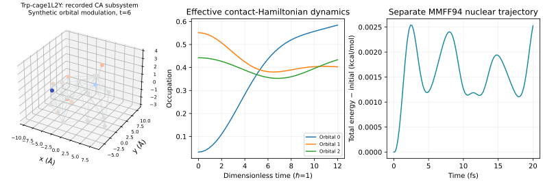
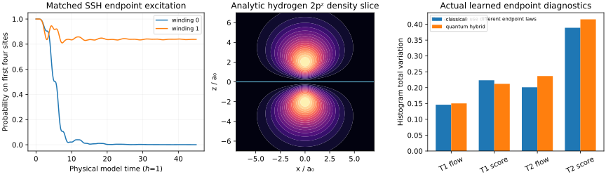
The complementary-data laboratory now separates deposited protein structure, actual finite quantum transport and learned conformation generation. Covalent bonds use explicit molecular graphs or qualified PDB templates, with depth ordering and visible atom/bond scales. The ribbon view reads deposited HELIX/SHEET records; short synthetic peptide backbones remain unassigned rather than acquiring invented secondary structure.
Five additional finite propagation examples compare matched SSH/QWZ topological and trivial controls and an SSH domain wall. Complex phase, probability, current, coherence and selected eigenstates are distinct views. Analytic hydrogen volumes illustrate nodes, quantum beats and a phase vortex; they are not molecular electronic-structure calculations. Eight further CPU runs train classical and two-qubit hybrid score/flow models on periodic MMFF butane/pentane torsion spaces. All checkpoints, losses, controls and positive noise endpoints are explicit. These examples neither establish quantum advantage nor close the independent arithmetic bridge for GRH.
An atomic coordinate cloud does not determine chemical bonds merely by looking connected. SDF graphs retain their explicit bond indices. For the PDB source view we select the first model, blank/A alternate locations and positive occupancy; solvent is omitted from the display. Standard amino-acid templates, explicit CONECT, qualified ligand/hydrogen proximity and geometrically valid peptide C–N links have separate provenance. The complete original file remains available. Display connectivity is not a newly measured bond label.
The parser follows the wwPDB3.3 record definitions [105]. A class-one HELIX is an alpha helix; class five is a helix, not another alpha helix. SHEET retains strand identity, sheet membership and parallel/antiparallel sense. Ribbon patches follow the actual CA trace and carbonyl orientation, with strand arrows and narrower coils. A peptide bond must connect neighboring residues before a patch or spline-control neighbor is allowed: spatially nearby disconnected fragments and TER-separated chains must not acquire a phantom ribbon. Regression tests include these controls. Backbone recognition in a short synthetic SDF peptide supplies a trace, not a DSSP assignment or evidence of a stable secondary structure.
The full-source geometry is distinct from the capped effective contact graph. In the full-source view, only mapped modeled CA sites carry its electronic field. Nuclear display interpolation adds no new integration steps. An NMR model index, a ribbon parameter and a generative time are not physical time.
For a finite Hermitian matrix and a normalized initial vector , the continuously evaluated browser state is
Unitarity gives . Differentiating gives and hence for . The actual complex one-particle coherence is . A common phase cancels from both current and coherence; node colors therefore use a stated phase reference. The probability height is a display encoding, not another physical coordinate. Current arrows are fluxes, not classical electron paths.
Two48-site SSH controls use the same initial endpoint orbital and exchanged strong/weak hoppings. Their periodic bulk winding is respectively zero and one for , with gap . A separate61-site domain-wall chain starts and ends with strong bonds and has two weak bonds adjacent to its central even site. Its sublattices have sizes31 and30. At zero energy, set the odd-site amplitudes to zero and solve the tridiagonal recurrence on even sites. The amplitudes decay away from the wall by the weak/strong ratio. The nonzero off-diagonal entries determine this vector up to scale, so the nullspace is one-dimensional. This proves a finite interface zero mode; it does not identify an arithmetic Hilbert–Pólya spectrum.
The QWZ examples have a rectangle and two orbitals per site. They use the same unfiltered corner spinor for masses and . Their bulk Chern numbers are and0 in the existing link-product convention; 32/64 meshes and gauge controls agree. Finite boundary probability, spectral weights and coherence remain measurements of the particular finite state, not definitions or proofs of that bulk invariant. Independent matrix-exponential checks reproduce the five propagated states. The hydrogen phase winding below, chemical torsion torus, dessin genus and persistent-homology classes are also different invariants.
In atomic units, take on the usual hydrogen domain. The displayed normalized eigenfunctions are
Their energies are , . The angular integrals and give their unit norms; opposite angular parity gives orthogonality of and . Consequently
has unit norm after removing its unobservable common ground-state phase. Its density has the interference term : this is the actual quantum beat shown in the volume. The radial node is ; the nodal plane is .
The state is proportional to . On a circle avoiding the nodal axis its phase winds once, and . Its current is and has an azimuthal component. This stationary density with nonzero current need not show a moving classical particle. A finite-radius ray-marched volume and its opacity/exposure curve are rendering choices, distinct from the analytic density and normalization. These are nonrelativistic isolated-hydrogen benchmarks, not many-electron molecular orbitals or ab-initio peptide density.
Butane has one selected torsion; pentane has two. All other internal coordinates are held at the recorded MMFF reference geometry. The finite grids have72 and points, respectively. At300K define
where the product wrapped heat kernel is used on and . Thus is an explicitly softened finite-grid Gibbs target. It is positive, smooth and normalized; it is not a full solvent or molecular-equilibrium distribution. No affinity, redox, efficacy or electronic-density label is inferred. The molecular animation rotates downstream atoms about each actual bond axis; its poses agree with independent RDKit dihedral assignments to numerical precision and preserve the bond graph and fixed bond lengths.
For the unit circle,
The product kernel gives and . A forward sample is . Conditioning the wrapped Gaussian mixture shows
Indeed, differentiate each image term and divide by the mixture density; the Gaussian score is the stated latent-noise target. Conditional least squares therefore identifies the marginal score. The implemented weighted DSM loss uses weight , not an unlabelled Euclidean proxy on cut angles. The periodic-input network is trained over the full normalized time interval.
With reverse clock , the ideal SDE is . Its Fokker–Planck equation at density is , as required. This connection to score SDEs is the standard method [106]; the periodic mixture here supplies an explicit control. Initialization is sampled from the actual , with , rather than silently assuming it is uniform. Sampling stops at , so the ideal endpoint is , whose Gaussian component variance is . It is not . The initial run exposed this distinction; its source and outputs are preserved. The corrected run uses the proper endpoint reference and no excluded small-time training interval.
Exact wrapped-mixture scores, finite-difference checks, nested64/128-step Brownian controls and stored learned trajectories accompany the experiment. A finite Euler diagnostic is neither a convergence theorem nor a guarantee that a learned score recovers equilibrium. Remaining noise and learned-field error are shown separately from the MMFF target.
Let be uniform on , independently let , put and . The cut locus has probability zero under these continuous laws. For every smooth periodic test function ,
This is the weak continuity equation with the correct uniform and endpoints. Writing , the conditional formulas are explicitly
Because is smooth and strictly positive on the compact torus, these integrals are jointly smooth through both endpoints and . Division gives a smooth bounded periodic with a uniform spatial Lipschitz bound. In particular by symmetry. The usual unique flow of this globally Lipschitz time-dependent field transports the stated marginals. Conditional regression targets and learns an approximation to , following the flow-matching and manifold formulation [107, 108]. Neither the regression loss nor a visualization replaces endpoint-error measurement.
The earlier seven-spin dessin experiment supplies an actual quantum Gibbs state and its partial trace; its learned circuits approximate specified state/field targets. The exact coarse action in the RG chapter is produced by integrating out physical spins. Here the chemical learner transports a classical probability law on internal coordinates. A quantum channel, an RG partial trace and a score/noise schedule are three different constructions, with different states, clocks and acceptance tests.
A concrete materials-design constraint already appears in the QWZ controls. Any continuous mass path from to passes through . The explicit bulk gap formula then gives zero gap. Thus such a generator cannot both change between these two Chern sectors and preserve the gap throughout that path. Sector-conditioned sampling, explicit transition states and gap/invariant checks are meaningful design tasks. Merely drawing a continuous latent interpolation does not meet them. The finite transport controls and the earlier learned thermal-state experiments provide distinct physics benchmarks for these requirements, rather than unverified predictions of a synthesized topological material.
Each hybrid has two re-uploading two-qubit layers: periodic angle/time encoding, trainable rotations and CZ, followed by eight actual Pauli expectations and a two-layer64-unit tanh classical readout. The angles and readout are trained together. Integer coordinate frequencies preserve periodicity of the measured features, and composition preserves it in the vector field. These are classically simulated quantum-feature hybrids, not coherent quantum chemical evolution or quantum-assisted measurements. The matched classical controls use periodic first/second harmonics and the same readout width. Parameter counts and individual seeds remain explicit.
Eight2400-update CPU runs retain heldout objectives, checkpoint weights, periodicity errors, independent Kronecker/Pauli calculations, parameter finite differences, exact-score comparisons and actual endpoint histograms. The limited runs do not establish quantum advantage. Flow and diffusion have different positive-noise endpoint laws and must not be ranked as though their targets were identical. Generative interpolation time is not molecular time.
The chemical torus is a concrete internal-coordinate space. Drawing it next to a dessin, a noncommutative torus or a Fukaya construction does not construct a functor or prove homological mirror symmetry. Likewise none of these finite learners constructs the missing arithmetic self-adjoint determinant bridge. Adding heat/noise is also distinct from integrating out physical degrees of freedom in the earlier actual RG chapter; a noise schedule alone is not an RG construction. New source, operator-domain, arithmetic and Lean obligations remain explicit.
Both datasets are additional public Parquet releases, with dataset cards, origin columns, source records, audit evidence and exact remote hashes.
Aster complementary topological response
Public Hugging Face dataset.
Default static rows: 16,384; separately labelled source-anchor rows: 576.
Verified dataset commit: 2b8ce36571298a3517b8c88bb23269341d9b8908.
Mora complementary conformer response
Public Hugging Face dataset.
Default static rows: 22,951; separately labelled source-anchor rows: 266.
Verified dataset commit: 53a6b66acaa69ef79584648f3f6dc068363c4837.
Use the pinned commit and configuration names from the dataset card; time frames do not
count as independent systems. The interactive explorer retains the full release receipts and
actual source-file downloads. No dataset was enrolled into either active model during this
work.
The data commits above remain immutable. Public visibility was enabled at the owner’s request on 4 November 2026, with new card-only commits recorded in outputs/publication/2026-11-04. No data file changed.
The density viewer now evolves spatial functions, including interference terms, instead of drawing independent spheres around occupied sites. Let be normalized real Gaussian basis functions, let be their positive-definite overlap, and set . For a Hermitian orthonormal-basis Hamiltonian and a matrix of orthonormal occupied columns, put
This density is nonnegative and has integral : unitarity preserves , and integration yields . The cross terms carry coherence. Replacing them by a sum of atomic densities generally changes the model. The displayed gain/loss field is , whose full-space integral is zero; positive and negative colors indicate redistribution, not particles with negative probability. Time interpolation of saved density frames is a display operation and is not an extra time-integration step.
For fixed-nuclei at separation , six normalized Gaussians (exponents at each nucleus) give an explicitly integrated one-electron Coulomb Galerkin model. We start in one normalized left-center Gaussian, then evolve with its time-independent Hamiltonian. The electronic ground energy is approximately Hartree; adding nuclear repulsion gives Hartree. This small basis is not a chemical-accuracy or basis-convergence result. Independent Coulomb quadrature, kinetic-integral and matrix-exponential checks pass.
The second example uses the deposited Trp-cage CA geometry, a specified twenty-orbital contact Hamiltonian and ten occupied model orbitals. Its spatial Gaussians have exponent . The resulting field is the exact density of this finite effective basis model, not a calibrated protein electron density, valence count or transfer-time prediction. The first example uses atomic units; the second retains its effective model time and length convention. These examples are separate from the fixed private dataset release and do not change its labels.
The viewer offers orbit/zoom, volume and isosurface rendering, time scrubbing, exposure and density/gain-loss palettes. The grid and 41 saved frames are encoded as 8-bit square-root-density atlases. The maximum decoded integrated-charge errors are electron for and model particle for Trp-cage; analytical full-space charge conservation is exact. Rendering thresholds, finite boxes and quantization are explicit display limitations. The separate hydrogen viewer retains exact analytic hydrogen orbitals and their coherent time-dependent superpositions.
ToricGT organizes graph tokens, trajectories and auxiliary algebraic data; its companion research program separates architecture, dynamics, memory, oracle labels and toric training objectives [143, 144]. This chapter extends that organization to the present surface-order problem. A quantum feature map can replace a specified finite feature block, and exact algebra can check a proposed relation or parameter. Neither operation supplies the arithmetic identification needed by Hilbert–Pólya.
The inspected ToricGT revision is a5199bc989a6fb170e21220e5e87bf95bc2fc0b4; the program revision is f91ba1811b5a4f70d53c7120acf8ca2a0049f85b. The files toric_algebra.py, tropical_toric_certificates.py, cas_certificates.py and the graph-token schemas are the concrete interfaces used here. Their mathematical objects are not inferred from repository names. In particular, we do not claim to have reproduced the upstream language-model training campaigns or their compression scores.
Let be the infinite polynomial elliptic-square dessin algebra of the preceding chapters. It has two quiver vertices, two arrows in each direction, and the specified locally gentle zero relations. Retain one arrow , put the other arrows equal to zero, and frame . Every path of length two now acts by zero, so these are genuine continuous finite-dimensional modules of the completed order as well. Impose the additional closed condition . In the chosen frames write
The coordinate ring is . This is a representation stratum with a rank condition; it is not an assertion that the full order or its invariant ring is a toric variety.
Proposition 35.1 (The Segre semigroup and its full relation). The homomorphism
has kernel . Its image is the semigroup ring generated by in . With all of degree one,
Proof. The displayed binomial maps to zero. Replace any factor in a monomial by until no such factor remains. The integer kernel of the exponent matrix is generated by in the order . Two distinct reduced monomials cannot have the same image: their exponent difference would be a nonzero multiple of this vector, and the monomial at the positive end would contain both and . Distinct reduced monomials therefore have linearly independent images. Reducing a polynomial proves . Multiplication by is injective in the polynomial domain , so the graded exact sequence gives the Hilbert series. In degree , image monomials are exactly with : choose the overlap of the -positions and -positions between and . This gives monomials. □
This supplies a small complete certificate rather than an unspecified “syzygy loss.” A learned output can be penalized by . After rationalization, checking exactly certifies the rank-one relation. It does not certify the learned point’s interpretation as a module with other nonzero arrows, an arithmetic endomorphism, or a positive spectral family. The multiplicative parametrization enforces this one relation identically, including degenerate rank-zero points.
The projectivization of this cone is the Segre surface . The full framed representation space, the rank-one cone, its projectivization and a quotient by the vertex group are different objects. Under the full left-right action on , its individual entries are not all semi-invariants. The determinant has its usual determinant character, but is identically zero on this stratum. Framing is thus part of the example, not an invisible choice of gauge.
The same square of exponents defines the max-plus function
Its corner locus is the union of the coordinate axes. There are four one-dimensional rays of weight one, with primitive outgoing directions . Their sum is zero. This is an exact local balancing calculation. The Newton polygon is the unit square.
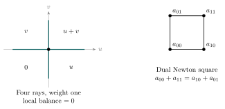
There are two associated tropical constructions, and they should not be conflated. The hypersurface of a four-term polynomial with this support lives in . The tropicalization of the two-term Segre ideal lives in and satisfies
The latter follows because the two terms of the binomial must have equal valuation. Over a valued field, tropicalization records valuations and initial degenerations; it is not a literal embedding of the tropical set as an ordinary algebraic subvariety of the complex toric variety. A fan specifies a toric compactification, while compatibility with that fan and the valued-field data specifies the relevant tropical geometry.
The inspected helper in tropical_toric_certificates.py uses integer supports, rational wall intersections and polygon edge normals. At this revision its input conversion applies int to floats. Consequently the exact claim here is restricted to inputs already verified to be integral; a nonintegral learned exponent cannot be silently rounded into an exact certificate. Pairwise ties also need their dimension checked. In the square example the pair ties maximally only at the origin, as does . These zero-dimensional sets are not extra facets. A balancing sum for one dual polygon is not by itself a certified Chow class on an unspecified complete fan, nor an exact description of a higher-dimensional tropical variety. The stronger boolean names in the upstream record are not used as additional mathematical premises here.
A useful hybrid pipeline learns affine scores with real parameters, exports integer/rational candidates with an explicit approximation rule, and then recomputes active cells, dimensions, weights and balancing exactly. The approximation error belongs to the learned model; the certificate belongs to the exported data. Recording both prevents a small floating residual from becoming an alleged exact identity.
The ToricGT shift convention differs from the forward shift used in some other chapters. At , with , its untwisted matrices act by
If are coprime they are a finite irreducible carrier of a central quotient. They do not faithfully represent the full rational rotation algebra. A boundary twist has to have modulus one if is to be unitary. Rational approximants to an irrational produce a sequence of finite models, but not an automatically nested sequence of matrix-algebra inclusions.
Proposition 35.2 (Ordered and symmetric Weyl multipliers). For integer pairs and set . Then
Choose a real lift of and set . Then
These formulas are on ; descent to exponents modulo requires retaining the resulting central phases.
Proof. Repeated use of , including inverses, gives and proves the first identity. The exponent introduced by the symmetric gauge is
Reversing negates this last expression. Dividing the two multipliers proves the commutator formula. Associativity also follows directly from bilinearity: for a third pair . □
The generic routine projective_phase instead evaluates . For skew its commutator phase is . To match the preceding symmetric gauge, use the explicit matrix
This factor of two and the orientation sign matter for learned phase features, circuit comparisons and transport around a surface. A separate numerical skew matrix is not automatically the ordered multiplier . For even , writing modulo would introduce another error; the real-lift formula avoids that operation.
For a density matrix , one physically measurable feature is
Its real and imaginary parts are expectations of the Hermitian operators and . They lie in . Thus a classical graph-token block can receive measured finite-dimensional phase features; a variational circuit can learn the state preparation or bounded observables; and a classical head can combine these with exact combinatorial records. No claim of quantum speedup follows from replacing an already inexpensive matrix calculation by a circuit.
Proposition 35.3 (A genuine positive feature kernel). For any finite list and any density matrix , the matrix is positive semidefinite.
Proof. For complex put . Then . □
This proof applies to a physical Gram kernel. It does not identify that kernel with a Jensen metric, the arithmetic explicit-formula pairing, or the determinant family of a completed -function. The latter comparison is an additional theorem, not a consequence of positivity of .
A typed record for a surface example should contain dart permutations, arrow endpoints, zero relations, central parameters, coefficient fields, module dimensions and category labels. Neural embeddings can be added to these records; they should not replace them. A candidate hybrid block is
where is a normalized classical attention rule, is prepared by a specified finite circuit, and is an exact certificate summary. Its architecture is meaningful even if the quantum features are first simulated classically, as in the finite training examples of the preceding computational chapter.
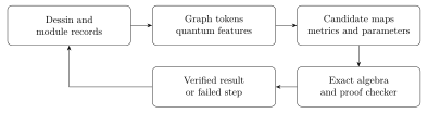
There are three distinct uses. First, supervised regression can learn a coarse-graining map against exact Ising or Gaussian targets, with a held-out parameter set. Second, a proposal model can search for a small module map or a polynomial identity, checked by exact substitution and stated presentation relations. Third, a proof-search policy can select candidate lemmas or tactics, whose accepted output must pass the proof assistant. Only the last two have the potential to yield new exact mathematical results, and only when the checker verifies the full exported statement. A classifier predicting that a proof is valid is not such a checker.
The ToricGT program’s certificate distinction is particularly useful here: store exact CAS data, validated surrogates and unavailable backends as different provenance classes. When comparing a quantum feature head with a classical one, hold the data split, parameter budget and objective fixed; report sample or simulation cost as well as error. A network with extra features need not improve the objective. None of the finite experiments in this book is an upstream full-transformer language-model ablation.
An exact candidate metric for a finite matrix illustrates the proposal/check distinction. For rational real entries, symmetry and all principal-minor nonnegativity can certify . Positive definiteness and then imply similarity to a Hermitian matrix: is Hermitian. Checking a few sampled minors or a small floating residual does not prove these assertions, and applying the result to an arithmetic family still requires uniform positivity and the exact arithmetic determinant comparison.
Kontsevich–Soibelman develop torus-fibration and homological-perturbation methods, including an comparison for specified subcategories of abelian mirrors [145, Sections 6–8, Theorem 4]. A lattice of phase labels is useful computational data for such geometry, but a finite Weyl pair alone does not construct either Fukaya objects or an functor. The latter must carry complexes of morphisms and all higher composition maps with their signs and convergence rules.
A concrete toric theorem provides a better model for the proposed link. For a smooth projective toric , Abouzaid constructs a full sub-pre-category of the relative Fukaya category of its Landau–Ginzburg mirror that is quasi-equivalent to the DG category of line bundles on [146, Theorem 1.2 and Corollary 1.4]. The theorem gives an embedding after the indicated derived/split closure; it does not assert an unrestricted equivalence for every non-Fano toric variety or for our singular completed order.
For intuition, the customary toric mirror potential for the Segre surface is
Solving gives , with critical values . The logarithmic Hessian is diagonal with entries and and is nonsingular at those four points. This is a direct calculation of a mirror potential. By contrast the two-level clock matrix has eigenvalues , since . The critical values and matrix eigenvalues are plainly different data. A proposal to relate them must specify a functor or quantization and its normalization; visual resemblance of their torus coordinates is not that comparison.
For gentle surfaces, the precise positive input already used in this book is the equivalence for a homologically smooth graded locally gentle algebra with its prescribed stopped surface and line field [66, Theorem 3.2.2]. Our nonempty closed dessin algebras have forbidden cycles and fail that smoothness hypothesis. A stopped quotient or categorical resolution can be a meaningful intermediate object, but it requires its own functor. Ordinary exact quotient inflation does not automatically preserve derived Hom spaces, AR triangles or determinants. In particular, the polynomial node branch has a valid stopped-annulus interpretation, whereas inflation into is not derived fully faithful, as proved earlier.
A finite training loss for or a chain-map residual checks only the displayed truncation. A genuine category construction additionally needs the remaining equations, admissible geometric objects, grading, compactness or convergence, and the claimed generation result. Tropical gradient trees can guide computations of compositions under appropriate geometric hypotheses; they do not remove those obligations. This is a constructive research interface: learn a small candidate, calculate its maps exactly, and then prove the specified comparison.
For the present Hilbert–Pólya program the useful learned outputs are candidates for arithmetic correspondences, controlled positive metrics, coefficient kernels outside the classes already refuted, or estimates with an exact symbolic witness. Every candidate must be checked against local Frobenius factors, central and deck actions, determinant multiplicities, conductor and gamma normalizations, and compact-uniform convergence on the stated complex domain. A Dirichlet comparison is not a proof for Hecke or general Artin -functions.
An exact finite witness can disprove a proposed universal construction, and that is valuable progress. A successful finite fit only proposes its next theorem. Neither a toric binomial certificate nor a positive quantum feature kernel proves that all arithmetic approximants have their zeros on the critical line. The small-gcd analytic estimate and the independent positive arithmetic determinant comparison therefore remain separate load-bearing research tasks. The role of the hybrid architecture is to make their search more explicit, testable and reproducible.
The executable example examples/quantum/toricgt_hybrid.py imports the pinned ToricGT rotation-algebra module. For it obtains four-dimensional Weyl generators and forms the Hermitian Harper family
A two-qubit PennyLane feature circuit and affine head, with twelve parameters, learn the smallest eigenvalue divided by six. Seed 20261104 specifies one hundred sampled couplings, with seventy-five training and twenty-five held-out samples. After 160 Adam updates the held-out mean-square loss is , compared with at initialization. These are finite simulated spectra, not -function zeros.
For six rational test couplings, the program forms the exact rational matrix
It rounds a learned proposal to a rational number and checks all fifteen nonempty principal minors of . A real symmetric matrix is positive semidefinite exactly when every principal minor is nonnegative, so an accepted proposal is an exact lower eigenvalue bound. A rejected proposal is repaired by rational bisection, starting from the independent Gershgorin lower bound and the Rayleigh upper bound . The saved rational minors certify the resulting lower bounds. Thus learning proposes; an independent exact criterion accepts or repairs. The certificate does not depend on the neural prediction being accurate. No arithmetic operator or completed-order equivalence is claimed by this experiment.
This benchmark has an exact closed-form solution: , so . For , rows one and three of agree, and the difference of rows zero and two is times row one. Thus its rank is at most two. Its trace is zero and , giving the stated eigenvalues (and hence characteristic polynomial). The experiment deliberately has an exact oracle: it tests learning, certificate acceptance and repair on a known problem rather than presenting a numerical fit as a new spectral theorem.
A persistence diagram records how objects and maps change under an ordered family of inclusions. A projective resolution records the generators, relations and relations among relations of one module. These descriptions meet naturally over a polynomial parameter ring. They must still be distinguished from the infinite locally gentle algebra attached to the surface: the parameter ring describes the filtration, not a replacement surface algebra.
The three supplied papers motivate these interfaces [147, 148, 149]. We use their surface-order, lattice and finite-presentation ideas with the corrections already proved in this book. In particular, a matrix satisfying consecutive-product zero is a complex, not automatically a resolution; Fitting base change is not exact base change; and the existence of a generic resolution is not a finite terminating algorithm. The worked example below proves its own exactness and exhibits an actual topological realization.
Let be a field and give its coordinatewise order. A persistence module is a covariant functor . Writing , put
Multiplication by and is the map to the next coordinate in the corresponding direction. Functoriality makes their square commute. Conversely the graded pieces and multiplication maps of an -graded -module define such a functor. General transition maps are multiplication by when . The exponents are nonnegative in this direction, a useful sign check.
This gives an equivalence for the stated discrete diagrams. Finite generation is an additional condition, not a consequence of having finite-dimensional pieces. A module can have infinitely many independent births. Finite cellular input with finitely many birth grades gives the finite presentations used here. A real-parameter filtration needs an appropriate discretization or a different coefficient algebra before being treated as a module over .
We write for a free module whose generator has grade . Over a field, a finite graded module has a minimal graded free resolution of length at most two. Minimality means that every differential entry belongs to ; tensoring with then kills the differentials. The numbers and grades of the surviving generators are the multigraded Betti numbers. The field hypothesis matters: has homological dimension three, and the regular sequence supplies a length-three example. The particular resolution below also works integrally, but that does not make every integral resolution length two.
Set
Its basis is , in grades . All other graded pieces vanish. The two nonzero proper transition maps send to and to . In particular, for comparable grades ,
This computes this module’s rank invariant; rank invariants do not in general classify all two-parameter modules.
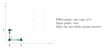
Theorem 36.1 (A minimal bigraded resolution). The following complex is a minimal graded free resolution of :
where
Proof. Each column of has the indicated source grade, and multiplication gives . If , its first and last entries give . Since is a domain, .
Suppose . Reducing modulo shows , say . Dividing the relation by and reducing modulo shows , so write . Substitution now gives , hence . Thus . This proves exactness at . The image of is its displayed ideal, giving exactness at and the augmentation. Every entry of both matrices has positive grade, so the resolution is minimal. The divisibility argument also works in , where remain prime and nonzerodivisors. □
The multigraded Betti numbers are consequently
They are dimensions of the corresponding graded . Taking degreewise Euler characteristics gives the same Hilbert series by two independent descriptions:
After forgetting the separate grading this becomes . The numerator records the alternating resolution shifts, not a characteristic polynomial whose zeros locate arithmetic -zeros.
One can also see the dual calculation directly. Ignoring shifts only to write the matrices, the dual differential is
The equations imply , again using coprimality. Thus . The second Ext is generated by with relations , and ; its -basis is . This keeps the syzygy calculation distinct from merely counting the support points of .
Start with one vertex and an oriented loop , both born at grade . Attach three two-cells by degree-one maps to that loop, at grades
At grade include precisely the cells whose birth grades are at most . Every boundary is already present, so these are actual subcomplex inclusions and their squares commute. The persistence cellular chain modules are
Therefore exactly. No assertion that every abstract persistence module has this particular geometric form is needed.
The loop survives before any disk is present and dies when the first disk appears. Two disks attached along their common boundary form a sphere. The first two persistent generators are the compatible cell cycles
Theorem 36.1 proves ; there are no three-cells to kill them. At all three disks give two independent sphere classes. Thus the same matrix is a relation among the killing cells and a positive persistent homology class in the larger CW complex. This auxiliary CW space need not be a Riemann surface: three disks along one circle are not a manifold. It is a topological realization of the filtration module, not another claimed cellular dessin.
Assume now , put , and let act on by linear substitution. The ideal is invariant. Its degree-two generators form , with basis . The linear syzygies form the kernel of multiplication
There is a natural equivariant map
Multiplication kills its image. On the two basis vectors its values are exactly the two columns of :
They are independent, and the kernel has dimension , so identifies it with . The Littlewood–Richardson rule gives
Here the partition convention uses symmetric rows. The equivariant total- graded resolution has multiplicity spaces in generator degrees . The diagonal torus recovers their bigraded weights and .
The grading distinction is essential. General substitutions mix and , so they preserve total degree, not the two original filtration coordinates. Only the diagonal torus preserves each bigrading. In positive characteristic the displayed maps and our exact resolution remain valid, but semisimple direct-sum representation theory must not be assumed. Nor does applying a Schur functor termwise to an arbitrary exact sequence preserve exactness, as the earlier counterexamples show.
For a finite presentation define
where is the ideal of -minors, for , and for . The ideal is independent of the chosen finite presentation. Its formation commutes with arbitrary base change because minors are polynomials in the presentation entries. For our cyclic module,
The support is the origin, but its Fitting scheme retains a length-three thickening. This is not the same datum as the rank invariant of the ordered graded pieces.
The -minors of are , so their ideal is also . Expected ranks are and this ideal has grade two; is a regular sequence. These facts agree with the finite-free acyclicity criterion of Buchsbaum–Eisenbud [150], independently of our direct proof. Over a general Noetherian ring, a height count cannot silently replace the criterion’s grade/regular-sequence hypotheses. The criterion concerns a finite complex over a commutative ring; it does not certify every infinite path-algebra resolution.
Arbitrary specialization does not preserve that exactness. At both matrices vanish, leaving positive homology in degrees one and two. More informatively, after setting only , the complex has
These follow immediately from and the two surviving entries of . They are the derived-base-change Tor groups. Flat base change, suitable Tor vanishing, or a new exactness proof is needed to obtain an ordinary specialized resolution. A generic parameter space and a small differential residual do not remove those conditions.
For variety language in this section take algebraically closed. Let have dimensions for . Fix feasible ranks with
The reduced variety
parametrizes based complexes with these upper bounds, not isomorphism classes of resolutions. Consider flags with , , and impose
Over the flag variety the allowed maps form the vector bundle
Its total space is smooth and irreducible. Projection is proper onto : for any complex with the rank bounds, first extend to a -plane inside , then extend it to an -plane there. On the full-rank locus the choices are uniquely , . Full ranks exist by feasibility, so this projection is birational. This proves the asserted incidence resolution of the reduced rank-bound variety.
For and , the two flag spaces coincide in a plane, and the base is . The vector bundle has fiber dimension and base dimension two, giving total dimension seven. Full-rank points are exact in positive degrees because and is injective. The zero pair is also a point of the complex variety and is not exact. Our polynomial matrices map the punctured plane to the exact locus; the origin maps to that nonexact boundary. A specialization of the universal matrices therefore still needs its own homological check.
Bruns’ generic-resolution construction uses a directed limit of rings which kills positive homology in the limit [151, Theorem 1, pp.35–36]. It does not assert that some finite stage always becomes exact, nor that every specialization of the resulting matrices preserves exactness. The finite example in this chapter makes its stronger local claims by explicit calculation rather than by invoking an unspecified generic object.
Return to the actual nodal interval dessin and distinguish its variables:
Both and are infinite dimensional over . The completed order is free of rank two over , on , with and . Multiplication by is injective, as is clear in its two normalization branches. Set . It has basis over , nontrivial arrow actions, and
is a genuine free resolution. The module is finite length, not a -free lattice. Its finite dimension does not turn its parent order into a finite-dimensional substitute.
The family is a persistence module valued in continuous -modules: each nonzero piece is , and its structure maps are the identity or zero as in Figure 36.1. The actions of commute with the fixed action of . There is no identification of either persistence direction with the order uniformizer.
More precisely put . Tensor the length-one -resolution just displayed with Theorem 36.1 over . Its finite total complex has free -ranks
and resolves . If denotes the order resolution and the persistence resolution, the total differential on is
Order the degree- terms as . Suppressing only the tensor symbols, the three matrices are
The cross terms cancel, so consecutive products are zero. For exactness, write a positive-degree cycle as , with and . Modulo the first component is a cycle in . That complex is exact in positive degrees, since tensoring vector spaces over is exact. Hence . Lift to in the free term and write . The original equation becomes . Multiplication by is injective on every free term, so . Consequently , as required. The same argument includes the top degree by putting missing terms equal to zero. Degree-zero homology is . This proves exactness without assuming that an arbitrary tensor product of resolutions stays exact. The ranks follow from .
This construction is compatible with the original center action. It does not shorten the infinite resolution of the nodal residue simple, make a lattice, or construct Frobenius. Restriction to the commutative coefficient ring doubles these free ranks. Determinant functors apply to the specified finite perfect complex, with virtual rank , but determinant multiplicity and arithmetic comparison remain additional questions.
An arbitrary time-varying interaction graph is not a bifiltration: an edge can disappear at a later time. One valid alternative fixes finite birth pairs for edges and includes an edge exactly when both coordinates are reached, then takes the flag complex. Another uses a cumulative union over times up to the first coordinate and decreasing interaction thresholds in the second. Both give inclusions; the second records cumulative history rather than individual snapshots. Vertices and higher cells must have compatible birth grades. Zigzag persistence is a different appropriate tool when deletions must be retained.
Quantum channels are linear on density matrices, but two unrelated channels need not commute. Assigning them to the two directions does not define a persistence functor unless the required squares commute. One may instead extract a declared classical correlation graph, choose a monotone filtration, and compute its homology with the conventions above. The data-to-distance rule and its statistical uncertainty still need justification.
For the research program this yields concrete trainable and checkable targets: propose birth grades, presentation entries or a low-degree syzygy; test inclusions, gradings, the matrix identities and actual exactness; record Betti and Fitting data before interpreting them. A loss penalizing checks only the complex equation. The exact module example, the flag-incidence model and the surface-order coefficient resolution show how to add the missing checks. None identifies those finite invariants with a completed arithmetic -function, provides a positive arithmetic spectral limit, or proves GRH.
The canonical on-page tool accompanies this chapter; other chapters link here. Proposition 2.3 generalizes the worked square-ideal resolution to every strict Artinian staircase. Four displayed ideals have lengths , with custom natural exponents also allowed. The tool shows generator and adjacent-syzygy degrees, standard monomials, exact comparable-grade maps and cellular incidence ranks. Coefficients in multiply field dimensions by four; the displayed free ranks over instead come from the cone. These are different rings.
Specializing the free resolution at a point over computes its fiber-complex homology. At the origin its dimensions are ; at each of the three nonzero points they vanish, since a pure-power generator becomes a unit. This is derived fiber data, not the CW homology at a filtration grade. The signed maximal minors and Hilbert numerator are checked independently with symbolic polynomials.
The quantum tab uses the single saved trained four-qubit QCNN unitary and the channel . The designed inputs have their last three qubits in . Their first qubit runs over eight equatorial states and both poles. This is an out-of-training-distribution illustrative family, not new training or a held-out performance claim. Birth labels are fixed from the input population : south , equator , north . They are retained at the output; recomputing them from output energy would not justify the same identity inclusion.
Floating-point input/output trace distances are scaled by and rounded upward. Their frozen integer graph labels are saved with a SHA-256 checksum and checkpoint provenance. The inequality of output and input labels is verified directly, never imposed by taking their minimum. Proposition 2.4 explains the exact-channel contractivity; the numerical records are not interval certificates. For the recorded labels, all finite boundary matrices and induced ranks are computed exactly over . At grade the input contains an equatorial 8-cycle and an isolated south pole, with . Its map to has rank one, whereas its map to has rank zero. The plotted two-parameter rank table fixes the target and varies comparable source grades; it is not a complete multiparameter barcode. Rotating the drawing changes the input-qubit Bloch layout only. The same layout is used at output and does not embed its two-qubit state space.
Independent row elimination and the browser’s bit-column implementation agree on both Betti numbers and inclusion ranks for the saved cases. These executable finite examples complement the proofs and the cited persistence theory. The worked square-ideal module now has a kernel-checked ungraded free resolution, described below. General staircase exactness, graded and categorical interfaces, the coefficient cone and channel norm contractivity remain separate formalization tasks. No learned component or finite homology calculation supplies the unresolved positive arithmetic determinant bridge.
The file PersistenceResolution.lean uses for an arbitrary field. Its free coordinate modules are and , with the matrices of Theorem 36.1. The augmentation is the actual -linear quotient map to . The proof of d1_kernel quantifies over all polynomial coefficient vectors; it is not a sampled scalar-rank test.
The reusable lemma relation_decomposition starts with a commutative domain and a pair such that and implies . From it constructs with . For the actual polynomial variables, the regularity premise is discharged by viewing as polynomials in with coefficients in . A polynomial is divisible by exactly when its constant coefficient vanishes; multiplication by the nonzero cannot kill such a coefficient. Thus the final kernel theorem has no unproved regularity hypothesis. The first and last coordinates then prove d2_injective; d1_range identifies the image with the specified ideal. Augmentation exactness and surjectivity complete the sequence, and the free terms are proved projective.
The field carries the residue action . The free modules retain ordinary polynomial multiplication. Both actions are explicit in the source, with action identities checked in the kernel. For every -linear map from the appropriate free term to this residue field, precomposition with or is zero, since all displayed entries contain or . These are actual Hom statements with their module actions, not merely entrywise evaluations. Abstract Ext-group identifications and the graded minimal-resolution interface are not yet packaged as formal theorems.
All theorem types and axiom dependencies are printed. Only the standard Lean foundations occur; no project axioms or incomplete proofs are used. This establishes the entire underlying ungraded worked resolution and its residue Hom differential calculation. It does not formalize every staircase, the CW model, Schur equivariance, the -coefficient tensor cone or any arithmetic determinant comparison. Those distinctions remain visible on the local verification page beside the executable laboratory.
For a primitive nonprincipal Dirichlet character , choose the completed -function with its parity, conductor and gamma factor fixed. A sufficient spectral program requires holomorphic functions on a connected domain containing the critical strip, compact-uniform convergence , and a proved zero-location property for every . A self-adjoint determinant representation must include its domain, determinant regularization, nowhere-zero normalization and coefficient comparison. Self-adjointness of an unrelated finite matrix does not establish any of these identifications.
If every is zero-free off the critical line, Hurwitz on each connected off-line component shows that the nonzero holomorphic limit is zero-free there. The limit cannot be identically zero on an open component if it is a nonzero holomorphic function on the connected containing domain. This last connected-domain hypothesis matters: componentwise convergence alone does not rule out an identically zero limit on a disconnected component. The conclusion is conditional until the arithmetic approximants and positive representation are constructed. General Artin functions also need their own holomorphy statement; Brauer quotients do not supply it. Hecke, Dedekind and elliptic-curve normalization and critical centers must remain distinct.
The original modular-geodesic argument fails at its prime identification. Integer hyperbolic traces and cannot match all rational primes. An asymptotic similarity between prime and geodesic counts does not give a termwise equality of Euler factors. Nor does finite-field purity for a family of curves prove number-field GRH. The local Jacobi theta construction is a positive arithmetic benchmark with its own coefficient and symmetry obstructions, treated in the earlier chapters.
Write . For squarefree primary column ideals of norm about , good away from a fixed set containing 2 and 3, let be the original sextic residue character extended by zero at nonunits. At the unit ideal take , including . For row-independent coefficients , the normalized Gram expansion is
For with squarefree and pairwise coprime,
The oscillatory primitive conductor is ; its zero-preserving periodic modulus is . Cancelling without its coprimality mask would change the row family. Möbius inversion gives
A row weight has to be evaluated at in this identity.
For a fixed nonnegative radial Schwartz profile , replace the sharp row cutoff by . For an off-diagonal pair, is primitive nonprincipal. If , its complete Gauss transform and lattice Poisson summation give, for every ,
Indeed the nonzero dual frequencies have Gauss modulus at most and the zero frequency vanishes. After scaling, Fourier decay bounds their sum by : for use planar annuli; for use a decaying power greater than two. The Poisson prefactor is . The ideal generator rotates and scales the Eisenstein lattice, so radiality preserves the profile in the divisor sum. This includes scales .
For , the mask costs , each kernel is , and there are pairs. Thus the off-diagonal normalized contribution satisfies
The diagonal is for . At , the dyadic range is therefore controlled by . The small-gcd range, especially , remains open. This result is for one fixed smooth radial profile; it does not prove the source’s stronger moving-profile or supremum uniformity. The derivation and surviving alternative routes are recorded in research/short-row-high-gcd.md.
Keep the original sextic family
with squarefree primary column ideals outside the fixed excluded set, their full annular coefficients (fix supported in ), and all nonzero Eisenstein element rows . The cubic symbol is , not . The following classical frame inequality [80] gives a new obstruction to one proposed estimate in this arithmetic program.
Proposition 37.1 (Coprime pair-square obstruction). Let be an -by- complex matrix with , and put . Then
For the original character kernels, let be the sum of over all distinct coprime squarefree column ideals in . At ,
In particular the proposed sufficient input fails for each fixed . This does not refute the signed Möbius mean square.
Proof. Set . Reordering four finite sums proves . The row diagonal contributes ; the column diagonal contributes . Removing the latter and retaining the former gives the inequality.
Restrict the column pairs in the nonnegative sum to distinct prime ideals of norm in , outside the same fixed set. If , no such prime divides a nonzero row element: divisibility would imply . Thus all original zero masks are exactly one on this ball, , and the residual primitive finite character conductor is , of norm between and . All these pairs have common divisor1. The lattice count gives . The classical unconditional fixed-field prime-ideal theorem gives ; this is an external analytic input, not a GRH hypothesis. At the stated endpoint , and the bound is therefore . □
To see the exact failed step, write and . Cauchy over coprime pairs bounds the absolute signed contribution by . The hoped-for pair-square upper bound would have closed this particular route, but is false. A large absolute pair-square mass is not a lower bound on the quadratic form with the fixed . Nor is the prime part a positive summand of the full Möbius energy: prime–composite cross terms can cancel. The original low-gcd estimate and the positive arithmetic determinant bridge remain open.
The finite matrix proof also retains an arbitrary row profile. Suppose for every column, set and . The row diagonals are and column diagonals are , so the same identity proves
This is a finite statement. Applying it to an infinite Schwartz tail would require its convergence and every newly encountered prime collision; these are not discarded. If a weighted pair-square attempt includes the annular , one can instead choose a closed subannulus on which a nonzero is bounded below. Its prime count still has order . The fixed has unit modulus outside its conductor. These facts do not replace the original coefficients in a signed estimate.
Here are exact sextic computations with all nonzero elements of the Eisenstein norm ball, and both prime ideals above each split rational prime in the column annulus. These kernel diagnostics use and exclude only primes above2,3; they do not compute a signed Möbius energy. Values are integer norms in .
| 128 | 4 | 18 | 22 | 6840 | 1584 |
| 1024 | 9 | 36 | 138 | 651672 | 506736 |
| 4096 | 81 | 300 | 456 | 60080328 | 21340800 |
| 256 | 64 | 240 | 40 | 363672 |
The final row has but ; its negative lower bound is correctly vacuous. The asymptotic theorem follows from the proof, not an extrapolation of these examples. For and in , evaluate as and take its power, lifting the six roots via . Every zero is tested before a unit value is assigned. For instance has norm7 and vanishes at modulo7, so the unimodularity hypothesis cannot be used beyond its stated domain.
ShortRowPairBarrier.lean verifies the finite frame identity, row-diagonal bound, weighted inequality and unimodular specialization, with actual complex sums and explicit hypotheses. It does not formalize the ideal-character comparison or prime-ideal theorem. The deterministic integer checker also verifies weighted profiles and256 scalar pair sums independently of its matrix computation. No numerical model or learned coefficient is used.
The next signed route must retain before Cauchy. An exact starting identity in ideal Dirichlet convolution is
Indeed implies . On squarefree , each divisor factorization retains pairwise coprimality; the original row zeros still multiply along it. Estimating these type-I/type-II kernels with their true conductors is a new open arithmetic task. The identity alone supplies no cancellation or GRH proof.
Keep the original squarefree good-ideal family, its fixed , its full and every zero-extended sextic symbol. In ideal Dirichlet convolution, write for every good ideal and let be the convolution unit. For put and . The classical Vaughan algebra gives
| (37.1) |
Indeed , and expansion of the last product proves the identity without an analytic assumption. This is a classical decomposition, not a new cancellation theorem; compare [87, Lemma4.1].
On squarefree all factors in are pairwise coprime. Define the actual, nonarbitrary coefficient functions
For squarefree , is times the number of the displayed ordered factorizations. For , . The two regrouped pieces are
Then . All ideals here remain outside the same fixed excluded set. The short term vanishes because and is supported in . No phase or coprimality mask was removed.
Proposition 37.2 (An all-cutoff separate-piece bound is false). Take the allowed principal , , and a fixed nonnegative smooth supported in , bounded below by a positive constant on a closed subinterval of of positive length. For each of the two pieces,
Consequently a proposed bound for each piece at fails for . In the exact original notation , it fails for . This refutes an all-cutoff termwise strengthening, not the original signed mean square or a specified moving-cutoff argument.
Proof. At , , so and . On the annulus the two coefficients are and , respectively. On squarefree ideals the latter is zero or two. At the actual unit row , every original character equals one. A fixed-field prime-ideal theorem gives good prime columns in the subinterval, so . Fix a good prime ideal . Products with varying distinct good primes in the rescaled subinterval have . Their nonnegative contributions give . Keeping that one row in each nonnegative energy proves the result. The prime-ideal theorem is a classical unconditional external input, with the field and fixed. □
The factorization does not shorten the primitive row conductor: for squarefree coprime it is , not or separately. For two resulting columns with common factor , the oscillatory conductor is and a zero-preserving period is . The signed low-gcd estimate and the independent positive arithmetic determinant comparison therefore remain open.
The monoid consists of nonzero integral ideals prime to the fixed excluded set . Every divisor of a good ideal is good, so the identity holds on this same monoid. Expanding convolution in (37.1) gives finite divisor sums. Multiply the identity by and sum. The extra squarefree indicator does not change , since . On its support forces each factor to be squarefree and any two to be coprime. Sextic multiplicativity, including zeros, gives ; a collision with any factor makes both sides zero. The fixed character also satisfies on these good ideals.
In the small-factor piece group . The remaining variable is squarefree and coprime to ; is necessary, but not sufficient for a nonzero : its specified truncated factorizations must still exist. For each such factorization on squarefree , , proving the coefficient formula. In the large-factor piece group . The condition implies , and summing that divisor gives exactly . Since , is not the unit ideal; its complete Möbius divisor sum vanishes, proving the alternative formula for . This regrouping never replaces the two-variable weight by , never deletes , and never replaces the resulting coefficients by a favorable arbitrary family.
One can instead keep the unrestricted convolution identity on nonsquarefree columns, but then both individual pieces and their local conductor description change. For and a good prime , the column contributes one to each of and , even though ; these cancel only after the pieces are recombined. Its squared sextic symbol has a cubic local component. Thus dropping total squarefreeness is not a harmless piecewise simplification, although the full unrestricted algebraic identity still holds.
For a squarefree with , every prime of has one nontrivial sextic local component in the row variable. Hence its primitive finite conductor is the ideal ; on the column support. On multiplying a column by the conjugate of another, the local exponent is zero at common primes, at a prime of , and at a prime of . The common prime still imposes its original zero on rows. Writing , therefore gives exactly
Here is the primitive oscillatory conductor and a period of the full zero extension. These are ideals, not necessarily squarefree rational norms. In particular, conjugate primes over one split rational prime are distinct coprime ideal factors. Full defining moduli of and primary conventions remain fixed in ; this row-conductor calculation does not assert a new uniform reciprocity theorem in the column variable. In the coprime bulk remains large.
On one type-II dyad let , , . Keep the full profile and coprimality restrictions in
The exact elementary Cauchy inequality is
The -mask has been kept inside . Even if one granted an optimistic uniform slice bound , the ordinary divisor estimate and the fixed-field ideal count would only yield the envelope
That hypothetical slice estimate is not established here. This is an insufficiency of the generic upper-bound calculation, not a lower bound on the signed energy. At balanced and , the term loses relative to the target; the term also exceeds . A sharper use of the actual , cross-factor constraints or covariance between the original pieces is required. This calculation does not refute all bilinear, moving-cutoff or dispersion methods.
The fixed- lower bounds in Proposition 37.2 are different: they are genuine energy lower bounds for the separate pieces. If on , count primes in for and in for . Removing and removes finitely many primes. The prime-ideal theorem gives positive constants times in both cases; the latter contribution has coefficient two. Because every coefficient of is nonnegative, keeping these products is valid. This is unlike isolating the prime part of the full signed Möbius energy, where uncontrolled cross terms remain. For the exact requested bound at , the competing power is , giving the threshold . Replacing by reparametrizes the loss and gives the equivalent formulation. The positivity argument is specific to . For a concrete control, the primary element has norm and three distinct ideal prime factors. At its type-I coefficient is , its type-II coefficient is , and its Möbius value is . Thus the separate pieces need not have nonnegative coefficients at another cutoff; no moving-cutoff obstruction follows from the preceding positivity proof.
The deterministic checker represents every good ideal of norm at most once by its primary generator, including inert prime ideals and squarefree products of three distinct prime ideals. It checks coefficient/regrouping cases at five cutoffs, retains encountered original zeros in actual sextic sums, and verifies pair-conductor exponent ledgers. It evaluates principal and the fixed Kummer character on the same good ideals. The finite diagnostic weight is the rational profile on , zero elsewhere; it is not claimed to be the smooth analytic weight of the theorem. Every identity is algebraic for arbitrary finite weights; these samples do not prove seminorm or scale-supremum estimates.
For example, at , , principal and , the unit-row normalized sums have the following exact common scaling:
Their exact difference is . The lower-bound theorem uses the prime-ideal proof, not extrapolation from these small numbers. An independent no-production-import oracle also checks convolution, squarefree regrouping and weighted sextic sums.
MobiusSplit.lean proves eight actual statements: the inverse-ring identity, natural-number arithmetic truncation/tail, the Möbius Dirichlet identity, the unit cutoff, its exact tail convolution and coefficient, and nonnegativity. The natural-number Dirichlet ring is an actual arithmetic object; it is not the ideal convolution ring. Ideal arithmetic, sextic/Hecke character construction, analytic prime counting and the unproved signed mean square remain prose or named classical inputs. No new zero-free region, full GRH proof or positive determinant bridge has been obtained.
The new Lean interface checks actual Plücker polynomials, nodal matrix relations and determinants, finite clock/shift identities and Kraus positivity/trace preservation. The short-row module checks finite-character masks, original finite Gram expansion, matched-row lower bounds and actual Eisenstein norm/evaluation identities. Full planar Poisson summation, ideal-character interfaces, the AR classifications, the derived functors and the complete physics program are not all formalized by these components. Their theorem types and axiom dependencies are printed in the verification logs.
The next load-bearing research task is an estimate for the remaining low-gcd original arithmetic kernel, or an independently constructed positive arithmetic determinant family escaping the precisely stated finite-kernel obstructions. A learned ToricGT-style component may propose a family, choose a search ordering or discover a candidate identity. Acceptance still requires exact algebra, analytic estimates, Lean interfaces where available and independent critical review. A fitted zero picture or a small training loss is an observation, not the desired proof.
We now continue the signed decomposition through its actual squarefree inner sum. Fix , the finite-order Hecke character , and the same finite excluded prime set , containing primes above and the conductor of . For , let be the primitive Hecke character induced by away from . It is defined before, and independently of, the type-I divisor . The abelian Kummer extension constructs the sextic factor; multiplying by gives the stated character. This uses classical abelian reciprocity, not general Artin holomorphy. Write for the primitive character inducing its square and for the two primitive conductors. For a squarefree good ideal put
All primes in are deleted even if absent from either primitive conductor.
Theorem 37.3 (Restoration and a uniform scalar contour bound). For the original type-I inner Dirichlet series is
It continues meromorphically to , with only a possible simple pole at when . In that case its residue is
Fix , and supported in . Set
Uniformly for , and ,
Here . The continuation and functional equation of degree-one Hecke functions are classical external inputs; the contour argument is given below.
At a good prime with , is ramified while its square is unramified; the second product in (37.3) must restore a factor invisible to squaring the zero-extended primitive value. At both characters can forget the prime, but the original row still vanishes on columns divisible by it. In particular, for principal , and at , the deleted local factors are
These are exact local calculations, not numerical evidence about zeros.
For , , insert into (37.4) and retain the actual and outer . Classical tame Kummer conductors give . Thus the normalized equals its displayed principal-residue sum plus an error with
| (37.5) |
The resulting elementary energy envelope is only
| (37.6) |
It does not prove the short-row target of order up to small losses. This is an insufficient upper bound, not a lower bound on the actual error or a counterexample to coefficient-sensitive averaging. The original signed mean square and positive determinant bridge stay open.
Let . Since contains , the extension is abelian, with character . At , arithmetic Frobenius gives the residue , exactly the source’s sextic symbol. Abelian reciprocity makes it a finite-order Hecke character; multiply by and take its primitive inducing character. The classical reciprocity input is [89, Theorem 0.8 and Chapter I,§1]. The finite-order archimedean character is trivial, since is connected.
At , write with a local unit. A sixth root of lies in an unramified extension: its residue root is separable and lifts by Hensel’s lemma. Inertia acts on a sixth root of through , so on the inertia character has order . It is trivial exactly when ; its square is trivial exactly when . A nontrivial tame one-dimensional character has conductor exponent one. Since is unramified outside , it cannot cancel this inertia there. At primes above , the groups are finite; their finitely many characters have a uniform maximum conductor. Consequently
The fixed ideal includes the wild and fixed factors. No assertion identifies with the larger full zero modulus.
For put . Its squarefree factor proves the ratio using the same deleted set in numerator and denominator. Restoring the primitive Euler factors yields (37.3). At a prime where the primitive square becomes unramified its value cannot be obtained by squaring the sentinel zero . For principal , has a quadratic Kummer character whose primitive square is globally principal. Its local value in that square is one, not zero. For both primitive characters are principal, although the full family still deletes . These two cases prove the local table directly.
For a character write for its Euler product with all primes of removed. For the product converges absolutely and is bounded by , uniformly in the character, and . Every deleted finite factor is nonzero there. Therefore
has just the stated possible principal pole. This uses absolute convergence at , not a conjectural zero-free assertion on the critical line. For any fixed and ,
Indeed for all sufficiently large ; the remaining finitely many prime ideals give a uniform fixed constant. This controls every moving deleted prime; the denominator has already been bounded by the full convergent zeta product.
We use the classical completed Hecke functional equation in the form
This is a named external theorem, not a newly formalized analytic result; compare [88, Theorem 4.3, Corollary 4.4]. The cited notes sketch some of Tate’s calculations; their incomplete displayed epsilon formulas are not used as independently checked constants here. At , absolute convergence bounds by . The functional equation and Stirling’s formula give on the bound up to a fixed constant. Phragmén–Lindelöf on this strip therefore gives, for fixed ,
For the principal character apply the strip argument to , then divide back on the fixed line . The constants need not be uniform as . Polynomial vertical strip growth and finite order, as supplied by classical Hecke theory, justify this application. No Lindelöf or subconvexity bound is inserted.
Initially, absolute convergence and compact smooth support give
Four integrations by parts using give . Choose , decreasing it further when distributing the small losses, and shift to . The convergent reciprocal Euler product, the finite factor bound and convexity above control the complete integrand. Their polynomial growth is integrable against this Mellin decay and makes the horizontal edges tend to zero. The only crossed pole is when ; evaluating its finite factors gives exactly . Taking absolute values on the new vertical line proves (37.4), after renaming the small losses. This also proves uniformity over any family of profiles with bounded ; it does not interchange a profile supremum with an arithmetic mean square.
In the original , the inner profile is exactly with ; no -dependent derivative enlargement occurs. On the support of , , hence . Also . The principal term is explicitly
This sum retains all original phases and zeros; no positivity of it is assumed. For the error use the actual truncated factorizations, not a free coefficient bound:
The fixed-field ideal count is ; dyadic summation proves the last inequality for sufficiently small . Inserting this and the conductor/radical bounds proves (37.5). The elementary lattice count then gives (37.6). Rows are not divided by units.
At and with , the power of the resulting error envelope relative to is
up to the arbitrarily small losses. It remains positive for every . Thus this scalar convexity argument alone supplies no short-row saving. This is a limitation of the estimate just derived, not an obstruction to averaging the numerators over Kummer rows, retaining signed coefficients, or exploiting covariance with type II.
The seminorm uniformity is not a proof of the original scale supremum. For each independently chosen scale the displayed outer argument requires . If a fixed cutoff is retained while shrinks, then eventually even : the short term in the Vaughan identity can meet the support and must be restored. Neither that term nor the covariance with type II may be omitted in a supremum or reassembly.
HeckeTypeI.lean checks seven actual complex local/finite-product statements, including independent primitive coefficient arrays and their full deleted-factor restoration. It does not identify an ideal Hecke series with an abstract finite product or formalize a Mellin contour. The exact checker includes split and inert prime ideals, actual sextic phases, conductor drops, sixth-power rows and original mask zeros. The analytic theorem above uses classical abelian reciprocity, Hecke continuation/functional equation and standard complex-analytic tools as external inputs. Full ideal-character/formal analytic objects, the original signed low-gcd mean square and every GRH completion obligation remain open.
Shared TeX sources: validated-oracle-core.tex · validated-oracle-results.tex · validated-oracle-details.tex · adaptive-readout-core.tex · adaptive-readout-details.tex · adaptive-theta-core.tex · adaptive-theta-details.tex · adaptive-family-core.tex · adaptive-family-details.tex · arithmetic-learning-core.tex · arithmetic-learning-details.tex · masked-moment-core.tex · masked-moment-details.tex · weighted-cutoff-core.tex · weighted-cutoff-details.tex · uniform-cutoff-moment-core.tex · uniform-cutoff-moment-details.tex · signed-bilinear-core.tex · signed-bilinear-details.tex · covariance-budget-core.tex · covariance-budget-details.tex · unequal-product-core.tex · unequal-product-details.tex · quadratic-pivot-core.tex · quadratic-pivot-details.tex · joint-gauss-core.tex · joint-gauss-details.tex · mixed-conductor-core.tex · mixed-conductor-details.tex · profile-uniformity-core.tex · profile-uniformity-details.tex · signed-weights-core.tex · signed-weights-details.tex · signed-divisor-core.tex · signed-divisor-figure.tex · signed-divisor-details.tex · rough-mask-core.tex · rough-mask-details.tex · coherent-main-core.tex · coherent-main-details.tex · physical-sieve-core.tex · physical-sieve-details.tex
Let , and , extended periodically, with parities . We approximate the completed functions The primitive theta/Mellin identity is the explicit classical analytic input; no hypothesis about zeros is used. These three examples do not assert a uniform result for all conductors, general Hecke functions or Artin holomorphy.
Theorem 38.1 (Scope of the supplied finite certificate). For each , the supplied exact-rational calculation constructs a complex polynomial of degree satisfying The computation includes enclosures of all true Fourier-circle nodes, completed-function sample error, analytic truncation, Fourier aliasing, the exact closed-form -step gradient-descent iterate and coefficient midpoint rounding. The Python implementation and informal analytic proof have independent checks; this is not a kernel-checked Lean theorem.
Proof. Write , with , , , . The independently recomputed rational theta majorants are strictly below , respectively, on . Use true roots and rational labels with proved error . Use the real Euclidean gradient on complex coefficient coordinates for Discrete Fourier orthogonality gives the least-squares optimum , , and gradient . For step and zero initialization, the exact -step iterate is . The code evaluates this closed form; it does not claim an explicit180-update optimizer run.
Set , and . Let be an outward rectangle enclosing and the sum of the coordinate halfwidths of the rectangle for . Choose each actual polynomial coefficient as that rectangle’s exact rational midpoint . The normalized basis is explicit: Thus the exported coefficient with index multiplies the normalized variable, rather than the raw power . Its error on the compact disk is bounded by Here is the sum of the maximum absolute real and imaginary coordinates, a safe upper bound for every enclosed complex modulus. Cauchy’s estimate and the Fourier identity for exact labels prove the alias and Taylor bounds. Label perturbations contribute at most per Fourier coefficient. The remaining two terms follow directly from the exact iterate and coefficient rectangles. Each term is rounded upward to a -bit dyadic rational; the reported total is the exact sum of those reported terms. The certified totals below are strictly below the asserted threshold. Detailed sample enclosures are proved in the extended edition and encoded with exact integer endpoints. ◻
| Conductor | Maximum sample radius | Uniform polynomial bound |
|---|---|---|
| 3 | ||
| 4 | ||
| 5 |
The displayed values are rounded upward; exact rational records establish the strict inequalities.
The final JSON records exact rational centers, interval endpoints, source hashes and all five error terms. Float values are display summaries only. A high-precision comparison is an independent diagnostic, not the reason an interval contains its mathematical target. Arithmetic uses outward integer operations, and invalid float/order inputs are rejected, including through typed caches. Earlier pilots and failed validation probes are retained.
This is a fixed finite tolerance/configuration. Increasing accuracy needs new truncation and precision choices; the fixed interface is not an arbitrary-accuracy oracle. The broader approximation existence theorem is separate. The certificate says nothing about the location of zeros: is not required to be real-rooted or a self-adjoint spectral determinant. The independent arithmetic determinant identity, positivity and original signed short-row/covariance estimates remain open. No GRH proof or complete new Lean4 formalization is claimed.
Real intervals are closed dyadic intervals with integer endpoints; complex intervals are Cartesian products. Addition is exact at this scale. For multiplication take the minimum/maximum of all four integer endpoint products, divide by and round down/up. For a reciprocal whose interval omits zero, reverse the endpoint order and round down and up. Negative denominators and scalar division use the same endpoint rules. Each operation encloses all represented real values by monotonicity; induction proves inclusion for every expression built from them. Rectangular complex multiplication uses these real rules. The sum of coordinate halfwidths bounds the complex distance from its exact rational center. Binary floating arguments are never silently converted.
For , the alternating arctangent sum and the endpoint obtained by adding the next signed term enclose . Sixty terms at and , together with Machin’s identity , give the interval for . The negative coefficient reverses the second interval. The identity follows from tangent addition and the range of the two angles; no decimal value of is a trusted input.
For rational , range-reduce , . With , The geometric tail bounds each remaining denominator below by . Use , the analogous expression for , and sign-aware interval multiplication by . This covers negative as well.
For complex , repeatedly halve until its interval magnitude bound is . The degree Taylor polynomial for then has remainder at most Successive absolute terms have ratio at most , so geometric comparison proves this bound. Add its symmetric interval to each coordinate, then square outward the required number of times. The identity and interval inclusion prove the final enclosure. Caches are type-sensitive: otherwise a cached exact argument can accidentally bypass rejection of an equal-valued float. No implementation change is allowed during the recorded run; the producer verifies source bytes again before emitting its certificate.
For the larger growth disk, , , take when and when . Both real Mellin exponents on that disk are at most . Define Integration by parts gives . The same Gaussian split and geometric-tail comparison used below, now with cutoff , imply the exact rational majorant Replacing the actual by the smaller positive increases the integral majorant. Exact fraction comparison gives , , . The producer recomputes these fractions, asserts the strict comparisons and exports them; the constants in the readout proof are thus checked rather than supplied by a floating growth estimate.
Let and . The standard primitive theta transformation, followed by splitting the Mellin integral at1, gives The second root-number coefficient is1 for these three characters: their finite Gauss sums are , and , respectively. For the last, ; the first two are direct conjugate-root differences. Division by gives the claimed normalization. Exponential decay makes the two integrals entire. This classical theta identity, not an assumption of Artin holomorphy or desired positivity, is the analytic input of the implementation.
The actual circle nodes are enclosed by computing with the validated primitives. All input boxes fit . Thus both exponents and satisfy , . The domain guard precedes all term discards. Retain and integrate .
Put , and . Since , for . Integration by parts gives . With , the omitted- tail of both integrals is Indeed , the function decreases, and . These inequalities yield a geometric bound after splitting the exponent in halves. The retained- time tail is at most It follows by substituting and majorizing by . The two tails are disjoint: omitted use the full integral, whereas retained contribute only .
Split each dyadic interval , , into four equal panels. For its midpoint and halfwidth , . For , , the principal logarithm is analytic on . On that circle, Here , and . The maximum handles both signs of . Cauchy’s coefficient estimate and cancellation of odd powers on therefore bound the error after degree by Indeed integrate each remaining even term, replace its denominator by the first omitted denominator, then sum a geometric series. Here . Multiply by for both Mellin terms and sum all panels and retained . Keeping this majorant even for later discarded terms only overcounts error.
To evaluate the polynomial stably, set , , and use Multiplying by and matching coefficients proves this recurrence, with . The integrated polynomial is ; all its arithmetic is outward.
Fixed absolute exponential-rounding errors can be amplified by high-order coefficients in late panels. The code therefore first bounds a complete pair, including both powers, by For real its phase has modulus1 and , proving the bound. If it is below , skip that pair entirely and add its bound to the final radius. This is controlled truncation, not numerical underflow. The final sample radius is the interval-sum halfwidth plus the omitted-, time, Cauchy and discard bounds. All are recorded separately and checked as nonnegative. No high-precision special-function routine is trusted here.
Run the preserved source on the existing Linux Python environment with no new packages: python3 on , with argument --output NEW. It refuses to overwrite an existing experiment directory. The final-v5 experiment contains samples, three rational degree polynomials, copied source and SHA-256 hashes. Independent validation checks rational endpoint arithmetic, transcendental enclosures, exact coefficient identities, high- precision completed-function comparisons and the exported component sums.
The fixed-parameter oracle solves a concrete evaluation/certification gap. It does not identify a positive arithmetic operator, force real-rooted polynomials, prove the signed original-family short-row bound or supply complete Lean4 verification. Surface/order and neural architectures may use these certificates as independent targets, but a small learned loss is not a substitute for the remaining arithmetic and categorical theorems.
The accepted final-v5 sample certificate is preserved unchanged. For each , it supplies rational complex labels , bounds , and outward rectangles enclosing the true roots , where , . The classical primitive theta/Mellin identity and accepted growth bounds on remain the analytic inputs. This extension accepts an exact rational error request on the fixed compact . It changes the finite readout, while retaining the certified sample errors and the -node alias budget. It is not an arbitrary-accuracy theta-sampling interface.
Theorem 38.2 (Executed rational readout with explicit refusal). For each supported conductor and rational request, the finite-data selection below either returns a normalized rational polynomial and an executed, exactly replayable gradient-descent trace with or refuses the request with the exact minimum base budget over all allowed degrees. Refusal concerns attainability by this particular fixed-data majorant; it is not an impossibility theorem for approximation.
Proof. Let be an outward rectangle enclosing , , computed from the preserved root rectangles. Put and let be the sum of its coordinate halfwidths. These are exact rationals, and . For a selected execute, using exact rational operations, This is genuine gradient descent with step for the explicitly specified real Euclidean objective , whose gradient is . All iterates and exact objective values are retained. The output is literally Set , , , and . The five budgets are Here . Cauchy’s estimate and true-root Fourier orthogonality give the alias and Taylor terms; certified label errors give the oracle term. Triangle inequality applied to gives the other two. Thus their exact sum bounds the compact-uniform error.
Define . Select the smallest with ; if none exists, report and refuse. For a selected degree, . Therefore executing updates until terminates after finitely many steps. The serialized coefficients, budgets, targets and trace use exact rational endpoints; displayed decimal approximations are not proof inputs. ◻
The original true-circle sample-label least-squares objective is With , Fourier orthogonality gives and the real Euclidean coordinate gradient . The executed objective instead has the exact rational midpoint target . The difference is enclosed coefficientwise by . Consequently this is an actual rational GD run for and a certified perturbed-gradient implementation for . It is not the exact optimizer trajectory of the ideal-root objective, nor a replay of neural or quantum training. An interval enclosure of an ideal-root GD trajectory would be a different explicitly labelled object.
Each actual update contracts by , so the exact stored losses satisfy . A replay recomputes every rational coordinate update, loss and weighted residual. The closed form is an independent check on the executed trace, not its producer. Exact rational loop coordinates introduce no further midpoint or floating export error. The arithmetic budget covers the difference between the certified Fourier rectangles and their midpoint targets, including the inherited root enclosure and outward interval operations. A subsequent float conversion requires its own exact conversion-error bound.
The normalized polynomial convention is essential: a stored coefficient with index multiplies , not . The input certificate is pinned by SHA-256, including its source hashes, all sample enclosures, root rectangles and analytic radius components. Producing source is captured at entry, checked unchanged before emission, and copied into a fresh output directory. An existing output is never overwritten. An independent replay should also check the fixed input hash, all dimensions, degree choice, the first stopping iterate, all five exact terms and their literal sum against the requested rational tolerance.
The attainable boundary of this majorant is Every request has strict budget slack for some degree and the proved finite stop rule. At or below that boundary this interface refuses. The degree minimizing need not be : Taylor error decreases with degree while the oracle and arithmetic sums increase. In particular and . Increasing the number of optimization steps does not lower these fixed-data budgets. Approximate boundary values on the stated compact are , and for ; only the exact exported rational minima are used for acceptance. These are certificate floors, not lower bounds on the actual errors.
A full adaptive theta oracle would separately need proof-preserving choices of omitted- cutoff, time cutoff, quadrature order, whole-panel discard budget, primitive series lengths, interval precision and serialized-bound precision. The present , , -bit arithmetic, primitive series lengths, discard threshold and -bit rounded budgets cannot support every positive request. Increasing a nominal bit count alone leaves the fixed primitive remainders and analytic tails in place. The preserved labels are not recomputed here. The classical identity, finite arithmetic and informal proof are not new Lean declarations. No zero-location, all-conductor, positive arithmetic determinant, quantum-advantage or GRH conclusion follows.
The interactive replay is available at the certified readout laboratory. All decimal graphics are illustrative views of the linked exact records.
For the primitive characters , , with parities , retain the classical primitive theta/Mellin identity and root number one already stated above. Put and . The following adaptive extension is implemented with independent interval and sample checks; it is an informal analytic theorem, not a Lean result.
Theorem 38.3 (Finite adaptive sample specification). For every supported conductor, exact rational , and rational , the choices below terminate and give a rational complex midpoint and exact rational radius with . The same conclusion holds for a specified true circle node when its root and node enclosures are refined on every precision retry.
Proof. For define the exact rational bound . Since , ; this bound is nonincreasing and tends to zero. Let and , . For , , , , use Here ensures a positive denominator; equals one for , so this safeguard is essential. On the four panels of each , write midpoint , halfwidth , , , and . Use the Cauchy remainder Choose in turn the first , first , and first for which their respective budgets are at most . Gaussian decay, then exponential time decay, then prove termination. These are the accepted tail and Cauchy arguments with each true exponential separately replaced by its upper bound .
There are potential pairs. A nonzero-character pair may be omitted only if its entire two-power contribution has bound Add every omitted bound to , giving . Evaluate all other integrated Taylor polynomials by the stated exact coefficient recurrence using outward rectangles. Refine both interval precision and all primitive series remainders until the final rectangle’s sum of coordinate halfwidths satisfies . For this fixed finite expression all input and primitive intervals shrink; continuity and outward arithmetic imply . Precision doubling therefore terminates, and the sum of the five raw components is at most . Choose an integer output scale such that and round each component upward by . The reported radius is their literal exact sum. With , it obeys The output retains exact rational midpoints, rounded components, , raw interval radius, parameters, input metadata and source hashes. The raw analytic bounds are exactly reconstructible; they need not be serialized as potentially enormous fractions. The output precision varies with the request and introduces no fixed reporting floor. ◻
This fixed-conductor sample result uses no hypothesis on zeros. It does not remove a downstream fixed-node Fourier alias floor, supply an all-conductor theorem or a positive arithmetic determinant, or prove GRH.
The primitive theta/Mellin identity with root number one yields On , both exponents satisfy and . For exact , put . The elementary inequality gives and . Use this solely as a pointwise nonincreasing upper bound; it is not multiplicative and has no asserted exponential integral identity.
Integration by parts gives for . For the bound is immediate. For , and give . For , the inequality therefore bounds the omitted- sum by Take ; then and the latter denominator is positive. Substituting in each retained- time tail gives The two tails are disjoint because the omitted- tail uses the whole integral and the time tail uses only retained .
For and take These panels cover and have . On , principal log is analytic, , and . For , the angular multiplier is at most , whence Cauchy’s coefficient estimate, cancellation of odd terms, and geometric summation yield the in Theorem 38.3. Including zero-character or later discarded terms in that sum is harmless. Gaussian, time, and geometric decay prove termination of the sequential first-success searches with . For fixed q and their asymptotic scales can be chosen as , , , and . Polynomial prefactors in contribute only to the logarithm of the error estimates; this is a truncation-size statement, not a rational-arithmetic bit-complexity bound.
For real , and . The bound for a whole pair, including both powers, is therefore . There are potential pairs; summing only bounds at most gives . No partial recurrence or isolated exponential is discarded. For active pairs retain the coefficient recurrence Coefficient comparison in proves that the integrated Taylor polynomial is Outward arithmetic encloses its exact value, including the signed character weight and both powers.
Use an isolated p-bit dyadic context, with all primitive remainders refined as p increases. Put . Each arctangent series separately stops when its next-term bound is at most , giving total weighted analytic tail width at most in Machin’s formula, before outward dyadic rounding. Each reduced logarithm series separately has tail at most ; for , the combined bound is , before rounding. For the complex exponential, after reduction to , choose the Taylor order so the bound is at most . Choose H by finite exact search; its denominator is positive. Add a symmetric exponential error enclosure to each coordinate before outward squaring. The fixed guard16 is not itself an acceptance bound: the final complete rectangle radius must satisfy . All interval caches must include p and preserve exact input-type guards. The successful p and retry precisions/radii are recorded. Individual series lengths are determined by these, the exact inputs and the pinned source and are reconstructible by replay; they are not explicitly stored.
For fixed N,J,K and exact target point, the expression has finitely many operations and only nonzero fixed integer denominators. Each primitive input is bounded for sufficiently large p; exponential halving counts are consequently bounded. Exact primitive tails and dyadic rounding widths tend to zero. Induction through the finite continuous expression, including finitely many outward squarings, gives . Doubling p after a failed comparison terminates. The argument also covers true roots and nodes regenerated at every p, since their widths tend to zero. A fixed nondegenerate s rectangle has no corresponding shrinking-input claim.
To justify convergence despite a growing exponential Taylor order, write , , and let be the sum of a rectangle’s coordinate widths and its magnitude bound. The rounded reduced input satisfies and ; the remainder is at most , so the first accepted order satisfies . For the computed term boxes, outward multiplication and integer division give and . Thus and ; adding the remainder increases width by at most . The pre-squaring width is therefore and its magnitude is bounded (indeed below for ). Each outward square has width at most ; the bounded number of squarings consequently preserves convergence to zero. Finally, exact rational partial sums and endpoint rounding give Machin width at most , and logarithm width at most for fixed . These estimates justify the primitive-width step without assuming a fixed Taylor order or asserting a global arithmetic complexity bound.
For serialization, initialize and increase B until . Write for each of the five raw components. Their exact reported sum is at most , and every component remains an upper bound. The output records B, the raw interval radius and complete rectangle, N/J/K, discard threshold/pair counts, exact target metadata and source hashes. These reconstruct all raw analytic bounds and pair sets without serializing huge exact tail denominators. For the practical requests below B is87 and114, respectively. Exact endpoints remain rational; the mathematical specification assumes an integer representation sufficient for the requested size. Dynamic rounding removes the old fixed reporting floor. For rational s, validate its exact coordinates in closed D before conversion: an outward dyadic enclosure of extends beyond D, but the analytic bounds concern the true point. Circle nodes satisfy the strict exact bounds , .
The exact parameter-design checker gives with exact rational budgets and no special-function oracle. The arithmetic precision is selected from the actual interval radius, not inferred from this table. This extension retains the existing classical theta identity; it adds no zero-location, positive determinant, all-conductor, Lean or GRH claim. The following end-to-end adaptive readout supplies its own node-count, alias, degree, Fourier and optimization choices.
The new driver changes the sample truncations, interval precision, circle size and degree; it does not reuse the frozen labels to assert a smaller error. Its scope is still the three stated primitive quadratic characters and the fixed compact .
Theorem 38.4 (Requested-error construction in the stated finite family). Given a positive rational and , the specified exact-arithmetic algorithm terminates in the mathematical unbounded-resource model and returns a normalized rational polynomial with Its sample enclosures, rational optimizer updates and all error budgets are explicit. This is an approximation theorem, with the stated classical theta identity as an input; it supplies no zero-location or positive determinant conclusion and is not a Lean theorem or a practical runtime bound.
Proof. Put , . Choose so , and choose so The driver rounds upward to a multiple of eight, which only decreases this bound. Set the requested sample error . The adaptive sampler gives all true circle nodes and labels with error at most . Form their outward Fourier rectangles through degree , and refine the nodes and finite evaluation arithmetic if their weighted midpoint radii exceed . This refinement terminates: for these fixed finite , node uncertainty and every finite-expression arithmetic width tend to zero with precision. Merely lifting fixed boxes would not suffice, so the driver regenerates the nodes and samples on this retry.
Choose rational midpoint targets and execute the previously specified quadratic-objective updates until . Their geometric contraction proves finite termination. The oracle, aliasing, Taylor and Fourier-midpoint terms are each at most , and the optimization term is at most . Hence the raw five-term sum is at most . Choose a serialization precision with , round each term upward, then add the five reported rationals exactly. The printed bound is at most . The polynomial uses , and the preceding Fourier/Cauchy proof gives its asserted compact-uniform bound. ◻
The trace is losslessly encoded by the fixed target vector and a rational scale extracted from each executed coefficient state, together with its objective, weighted residual and full-state hash. Every coefficient can be recovered exactly; a separate replay expands the states and checks every update. The producer does not generate its trace from a closed form. The saved objective remains the rational Fourier-midpoint quadratic, with its perturbation from ideal-root least squares explicitly budgeted.
The degree and circle-size choices use only rational comparisons. Since , the Taylor test succeeds at finite ; since , the alias test succeeds at finite . The common growth bound10 is safe for all three families; the certificate also recomputes the previously proved exact conductor-specific majorants below .
At fixed , the analytic truncation parameters are fixed while precision is doubled. The computed sample centers stay bounded: their underlying finite expression is fixed and the true completed-function values are bounded on the sample circle. Its arithmetic widths tend to zero, as do the regenerated true-root enclosures. Fourier computation is a finite composition of additions, products and division by the positive integer . Its midpoint-radius sum therefore tends to zero. This proves the driver’s additional precision retry, without pretending that changing a box’s nominal precision shrinks its uncertainty.
The accepted sampler error may remain above its actual arithmetic width because its analytic tails and output bounds are fixed for this . That causes no problem: the oracle allocation uses the total certified sample radius, whereas the Fourier-midpoint allocation uses only finite coefficient-rectangle width. No analytic sample error is silently moved into the latter term or removed by numerical convergence.
For the stored training trace, the exact loop gives from . Inductively every state is a rational scalar multiple of the same target vector. The producer first executes the actual vector updates, then extracts this scalar from a nonzero target coordinate, checks all coordinates, and records a canonical full-vector SHA-256 hash. If the entire target vector is zero, its zero state needs only scale0. The compressed record is thus an exact representation of the executed states, not a floating-point sketch. Hashes are integrity aids; exact vector reconstruction and the independently checked recurrence establish the mathematical claim.
Coefficient export uses exact rational numerators and denominators. A chunked decimal integer encoder/parser handles endpoints beyond Python’s usual digit-conversion guard without changing global interpreter settings. No fixed -bit serialization floor remains. The decimal graphics are separate approximate projections, not polynomial coefficients to which the exact certificate may be applied without a conversion-error bound.
All producing source bytes are captured, copied into fresh output paths and checked unchanged. Historical fixed producers are pinned and untouched. For the new modules the run also checks the import-time source snapshots, so a stale imported module cannot be attributed to later source bytes. After output creation, a failed evaluation, final provenance check or serialization emits uncertified failure metadata. Invalid requests and stale import-time sources are refused before creating output artifacts. Old outputs are never overwritten. Extreme requests can be computationally impractical: the termination proof gives no machine-time or memory guarantee, and finite test runs establish only their reported cases.
Nothing requires the output polynomials to be real-rooted, to equal an arithmetic Fredholm determinant, or to have a self-adjoint realization. Consequently arbitrary compact approximation of these known functions does not imply GRH. Uniformity in changing conductor, general Hecke/Dedekind/ elliptic/Artin scopes, the independent determinant comparison, and actual analytic/category Lean objects remain separate obligations.
The unsigned refinement in Section 40.15 leaves a signed problem. Here is a separate, executed finite learning objective on the original correlations, with a certificate for every coordinate and observable. It is not a uniform estimate for an expanding family. For ordered distinct squarefree columns , put and The symbols vanish at every collision with ; the common-prime mask is retained separately. With principal , actual complementary divisor counts , and one common complex profile , define The exact diagonal and these offdiagonal coordinates give (38.1) Thus and for the actual normalized row sums. Neither the Möbius sign nor a complex conjugate is discarded.
Proposition 38.5 (A finite supervised certificate). Let be complex readout coordinates and . For and , the substituted readouts satisfy The executed metric-gradient update gives . Therefore every positive rational requested tolerance on these three squared bounds is attained after finitely many updates on this fixed exact instance, with unrestricted resources.
The implementation’s resource guard refuses requests beyond its update budget; termination in this proposition is not a practical runtime guarantee. The labels are computed exactly before training, so no speedup over exact label evaluation or generalization to unseen conductors is claimed.
The supplied instance uses , above , principal , and all good squarefree ideal columns at activated norms (respectively ideals). One explicitly specified common smooth four-bump profile is zero at every other integer norm. Both the literal rows and the separately labelled guaranteed nonprincipal subset are evaluated; the latter is not asserted to be the whole nonprincipal family. There are offdiagonal blocks, with , and ordered learned coordinates. Every row case retains raw column zeros. Real and complex profiles give four requested- certificates, using metric updates respectively: executed updates, with every full rational state saved. A separate executed ordinary coordinate updates are budget-limited and carry no requested-error claim. The standalone replay is linked from the book and project page. No analytic saving, positive determinant, zero-location assertion, upstream quantum training, new Lean declaration or GRH conclusion follows.
For each block let . A literal admissible row determines local phases at every prime of ; rows with a -collision or a common-prime collision with are deleted before forming the exact sparse histogram . Orientation has Different active orientations have distinct exponent vectors modulo , so their characters are orthonormal for the uniform measure on . The model and target projection are Indeed is the orthogonal projection of onto this character subspace, and . The positive spectral metric assigns weight to this orthonormal basis. Its squared error is exactly . Thus the run evaluates the full finite feature-projection loss by Parseval; it does not claim to have executed a sampled or stochastic training loss. This projection need not be a nonnegative density. A Hermitian readout matrix need not be positive semidefinite.
Use coordinates , so and . For the objective , the ordinary real-coordinate gradient in block is . In the block metric , the gradient is . A metric step of size therefore halves every complex error and quarters . Conjugate initial coordinates and this step preserve the Hermitian reverse orientations. The ordinary trajectory treats all ordered coordinates independently; asymmetric weights need not preserve that symmetry. For ordinary steps , the Hessian eigenvalues lie between and , whence This last bound is conservative; the saved ordinary steps per case are not asserted to attain the requested tolerance.
Proof of Proposition 38.5. Subtract (38.1) with the same exact diagonal. Weighted Cauchy–Schwarz, applied only to the error, gives Here because is squarefree; the predicted sum itself keeps its signs and phases. Each summand in the second factor is nonnegative, which proves the coordinate bound. The exact affine update gives , proving contraction. For finite rational positive and , some integer makes all three bounds at most . The zero-error case stops immediately. No varying-family constants enter this finite assertion. ◻
Let These disjoint bumps are supported in and . For the real case ; for the complex case . At integer norms at the four activated norms and is zero elsewhere. Hence all active original squarefree columns are present, rather than an undeclared column submatrix. No exponential evaluation is needed at these exact nodes. The profile is a fixed finite demonstration and does not establish a profile-uniform analytic estimate. The counts are at the four norms. The guaranteed nonprincipal subset removes precisely those literal rows whose outside- norm is ; no classification of the omitted rows as a whole is asserted. Every nonunit outside- factor has a prime exponent from to , since its prime norm is at least and ; its nonzero residue modulo gives a nontrivial local character. All six units and all original -power rows belong to the separately saved full literal case.
The seed selects deterministic rational conjugate initial coordinates by SHA256 of the ordered column identifiers. There is no random sampling. Exact arithmetic stores every metric and ordinary state. Training accepts only when both observable certificates and the uniform-coordinate certificate are at most , preventing a scalar cancellation from masquerading as accurate correlation learning. The real full-row targets are and ; the guaranteed-subset targets are and . Complex-profile targets and the complete phase histograms are saved alongside. Each case has nonzero negative- C–C target orientations. Replacing all signs by plus is an explicit failing control, not an estimator.
The complete run is reproducible.
The source is examples/arithmetic_learning/learn.py; its README states the exact smooth profile, CLI, resource guard and loss convention. The accepted immutable output is outputs/experiments/2026-11-05-arithmetic-learning-v2/. All source/helper hashes, exact input bytes and artifact hashes are bound before and after execution and checked on replay. Existing outputs, nonpositive or binary-float tolerances, and stale source/input/case bytes are refused. The preserved v1 logging failure is not the accepted run. The focused verifier independently reconstructs local symbols and Gram targets, then checks the full saved metric trajectory. Independent mathematical review and exact code checks are recorded separately; finite arithmetic checks are not a proof of an asymptotic signed estimate. Full exact training labels are supervision, so this is a certified finite reference architecture, without an efficiency, generalization, PSD, zero-location or GRH claim. Analytic and categorical Lean remain unfinished.
Let , , and write for the ideal or element norm. Fix a finite-order Hecke character and a finite set of prime ideals containing those above and those dividing its conductor. For , let be the character of defined using arithmetic Frobenius, and put . Here means the underlying primitive Hecke character: it is formed before introducing any divisor variable or evaluating conductor-dependent zero extensions. The rows below are all actual Eisenstein elements, including units and prime powers supported in .
The external inputs are abelian Kummer reciprocity and character uniqueness, the primitive Hecke functional equation and its usual vertical growth, Stirling’s formula, scalar Dedekind-zeta convexity, and Blomer–Goldmakher–Louvel’s large sieve for their specified sixth-order family. We use the pinned arXiv:1112.1650v1, Theorem 1.3, Lemma 2.1 and Appendix II; its Section 5 supplies the all-ideal decomposition whose fixed-twist proof is redone here. No statement about all primitive characters of comparable conductor, Artin holomorphy, Lindelöf bounds or zero locations is assumed.
Theorem 39.1 (The original-family numerator moment). For every , uniformly for and , (39.1) For every fixed , the same estimate holds with replaced by , with the constant also depending on . If the central bound has constant at an exponent , an admissible off-central constant is (39.2)
Proof. For the canonical BGL character , Appendix II gives a radicand with . Since is principal, comparison with any literal whose outside- ideal is gives for one of finitely many fixed -unit Kummer twists . This is an equality of primitive characters, established outside a finite set and extended by uniqueness. For each outside- ideal and -supported integral ideal , at most six elements generate . The resulting -supported multiplicity sum converges at exponent .
For each fixed , split the canonical parameter as , where is squarefree, is squarefull and sixth-power-free, and . The primitive conductor is at most a fixed multiple of . The common-gamma approximate functional equation, with and , has common maximal length for any sufficiently small fixed . Mellin inversion removes its row-dependent conductor weight. Split a column as , with supported in , squarefree and squarefull, the last two coprime and prime to . The original primitive values at remain bounded row multipliers. The -supported and squarefull column weights are summable at . Multiplying squarefree column coefficients by the fixed preserves their squared norm, whatever its finite order. BGL’s large sieve therefore bounds the energy for fixed by Squarefull counting and summation give . The sum converges at exponent . Principal rows are separated before the pole-free functional equation and bounded by scalar zeta convexity. This proves (39.1).
For the off-central statement divide each by and, on principal rows, also multiply by . These are bounded analytic functions on , continuous on the boundary. Poisson representation and Jensen’s inequality transfer the central squared moment. The convolution of with is at most eleven times that weight when . Restoring the denominator and the principal pole-removal factor gives (39.2). The extended edition gives the detailed derivation with all primitive local values. ◻
The moment theorem also holds for any one fixed unitary Hecke character . For precision choose , with angular parameter and completed gamma factor All finite Kummer twists have this same infinity type. Use , comparable to with -dependent constants. Pure norm rows have and are separated before the pole-free functional equation; their pole at is removed by . No uniformity in , or the conductor of is asserted. This extension of the moment is separate from the following finite-order type-I residue formula.
Retain the original zero-extended symbol on good squarefree ideals. Let be the ideal Möbius function and set Let , formed independently of squaring any zero sentinel. With and the primitive conductors, the full-mask series is (39.3) Initially it equals for . Every prime of remains deleted, including those forgotten by either primitive conductor.
For finite-order , , , , and supported in , put On , the exact residue-subtracted type-I remainder is (39.4) This definition retains the actual , all phases, -masks, conductors and the independently primitive square.
Theorem 39.2 (An improved masked residual estimate). Under the preceding finite-order hypotheses, for every , (39.5)
Proof. The same deleted set in both factors of (39.3) gives : the reciprocal incomplete Euler product at is bounded by , and its remaining finite numerator is bounded by a small power of its radical. Apply Minkowski to (39.4) in the exact row space and use Theorem 39.1. The actual coefficient sum is at most Four Mellin integrations by parts bound the remaining height integral by a constant times . Square the result and absorb the small losses using . ◻
At and with fixed , the upper bound’s excess over is , up to small losses; as it still leaves . This is a limitation of the upper bound, not an energy lower bound. The extracted principal residue, the original short term at smaller scales and the signed type-II minus type-I covariance are not controlled by (39.5). The next arithmetic task is to estimate the complete -weighted moment before its absolute coefficient sum, or establish sufficient signed covariance. No positive arithmetic determinant, zero-location theorem or GRH proof follows. The analytic argument uses the external classical inputs above; finite diagnostics and selected existing Lean local identities do not formalize the Hecke functions, approximate functional equation, Poisson transfer or these moment bounds.
We prove the analytic statements of Section 39.1 from the explicit classical inputs stated there. Write for the nonzero integral ideals prime to , and for the ring of -integers. Constants may depend on the fixed field, , and any declared positive small exponent. No such constant is asserted uniform in the conductor or infinity type of a varying .
Use Appendix II of BGL, with . Its fixed local modulus and representatives may be chosen once, since contains the primes above and has class number one. For each the construction writes so . Choose generating as an -ideal. If , then There is a precision here: Appendix II allows choosing relative to a tested denominator. Fix one admissible global decomposition first. Its radicand gives the canonical character on all primes outside the finite set where that choice applies. Uniqueness of Hecke characters, equivalently Chebotarev in the finite abelian quotient, then identifies the underlying primitive characters everywhere. With matching arithmetic-Frobenius conventions, (39.6) If the residue-symbol convention is conjugated, conjugate the canonical family and its coefficient sequence; the same large sieve follows.
The group is finite. Thus (39.6) uses one of a finite set of fixed Kummer twists , all unramified outside and of bounded -conductor. This is a comparison of primitive characters, not a pointwise multiplication rule for independently zero-extended arrays at bad primes. In particular, a conductor drop must not be replaced by a product of artificial zeros.
Since is principal with six units, for fixed and an -supported integral ideal there are at most six satisfying . For any nonnegative row quantity, the literal moment is consequently at most (39.7) An ideal bound therefore transfers to all literal rows, since No quotient of the original unit rows or deletion of -prime powers has occurred.
Fix and write . Its fixed conductor is supported in before the Kummer twist. On columns prime to , . BGL Theorem 1.3 thus gives, for any fixed , (39.8) The first fixed multiplier preserves the coefficient norm; the second has modulus at most one. Restricting the positive outer row sum is harmless. A coprimality condition with another fixed ideal belongs to . In particular, need not have order dividing six and is not asserted to belong to BGL’s finite ray-class character set.
There is a unique valuation decomposition Indeed, for , , put the residual prime in if , and its exponent in if . BGL Lemma 2.1 gives and on ideals prime to in this sixth-power-free case. Those are the identities needed here; no arbitrary multiplicativity assertion is substituted.
At a prime outside , tame Kummer inertia at residual exponent has order . It is nontrivial for and has conductor exponent one. The fixed is unramified there, so cannot cancel that inertia. At primes in the local sixth-power classes are finite, hence only finitely many primitive conductor types occur after multiplication by the fixed . Consequently (39.9) independently of . The equality of the conductor’s outside- part with does not identify that conductor with the original larger deleted set.
First take finite-order . All characters then have trivial infinity type at the complex place. The primitive completion may be normalized as For nonprincipal rows the completed function is entire. Apply this functional equation to the Mellin integral with even auxiliary factor and denominator , shifting across . At this gives two weighted Dirichlet series, truncated below to polynomials; the dual prefactor has modulus one. Principal rows are excluded from this pole-free step and treated separately below.
For fixed , let and . An explicit normalized kernel is (39.10) with small. Its factors combine to in the actual completed-L kernel; there is no extra factor of . The denominator supplies the residue at zero. On , Stirling and give The factor makes this an integrable majorant uniformly in . The analogous bound holds on every fixed positive shifted line and for the dual gamma kernel. Moving far enough to the right gives arbitrary power decay beyond a common total-ideal cutoff (39.11) up to fixed constants. For any requested , a sufficiently large positive kernel shift, depending also on , makes the truncation error uniformly in all rows in this block. Ideal counting bounds the absolute tails. Such errors are negligible after the finite row sums by taking larger if needed.
Insert (39.10) on . The factor is independent of the column and is a row multiplier of modulus at most . Its imaginary part is a phase. The remaining column coefficient is , apart from fixed constants. Minkowski or Cauchy with the integrable gamma majorant therefore removes the row-dependent weight at cost in the squared norm. No independence of the root numbers is assumed or needed.
For each column use the unique decomposition where ; a prime of outside- valuation one goes in , and a prime of valuation at least two goes with its full exponent in . For fixed retain as the original primitive row value. On the good factors the exact canonical identity applies. The remaining factors involving , including , are bounded row multipliers. Their moduli are at most one; only then are they discarded in an inequality. In particular the value at is not replaced by the product of zero-extended primitive arrays.
For the polynomial the coefficient sequence is independent of ; it includes the indicator and the common cutoff . Padding it by zeros up to is legitimate. Its squared norm is at most . Minkowski over is legitimate because The finite Euler product handles ; the squarefull series converges above . Apply (39.8) to each such polynomial and to the conjugate dual family. For fixed the resulting energy is (39.12) The additional condition simply restricts the positive row sum. The large-sieve small exponent can be chosen sufficiently small along with and absorbed in the indicated small loss.
Every squarefull ideal has a unique expression with squarefree. This follows primewise by using exponent zero or one in according to the parity of an exponent at least two. Therefore For the count, sum and use . Summing (39.12) over gives since the squarefull series converges at and , , and for . The sum is bounded by . Choosing all internal losses small for the requested final proves the fixed-twist all-ideal central moment.
There are ideal rows in total. On any row where the primitive character is principal its -function is , and ordinary scalar convexity gives . This treats those rows without a pole-free approximate functional equation. Finally (39.7) proves (39.1) for every actual nonzero Eisenstein element.
For a nonprincipal row define using the holomorphic logarithm on . On a principal row additionally multiply by . Analytic continuation and ordinary degree-two convexity, used separately at each fixed conductor, show that is bounded analytic on the right half-plane , with continuous boundary and decay at infinity. The principal pole is removed before applying Poisson representation to its real and imaginary parts. Jensen gives The exact row family is finite for fixed , so its sum interchanges with the integral without a limiting-family issue. The boundary pole-removal factor has modulus at most one.
Take and . Since , the central squared moment of the is bounded by , where . For , split from its complement. The near contribution to is at most . In the far region use and , giving at most Here for . For , the convolution is at most one and hence at most . Thus uniformly for . Restoring the denominator costs less than , and the inverse principal factor is bounded by . The product proves (39.2). The constant is uniform as , but not as the contour approaches the principal pole line . No zero-free hypothesis appears.
Let be fixed and unitary, with angular parameter and gamma factor stated in Section 39.1. The external primitive functional equation is explicitly A constant norm-twist phase in another completion convention is absorbed in . All finite Kummer twists share this infinity type. Replace in the kernel by . The numerator gamma ratio now has real base and vertical parameter ; its conjugate dual has parameter . Stirling gives the same integrable Gaussian-majorized kernel on each fixed shifted line. Constants can depend on ; is comparable to for this one fixed . The finite-prime conductor analysis, modulus-one coefficient twist, all-ideal decomposition and all original primitive row values remain unchanged.
A pure norm row has ; exclude it from the pole-free approximate functional equation and use scalar convexity at . In the Poisson step cancel its actual pole by This factor is analytic in the relevant right half-plane. On its boundary , while inside . Hence the same transfer factor applies to the now -dependent central constant. If the opposite norm convention is chosen, replace by in the gamma factor and pole alike. This proves the separate fixed-unitary moment assertion; it does not claim uniformity in a family of infinity types or replace the finite-order principal-residue expression below.
For , define by removing every prime of , not just conductor primes. The identity (39.3) is equivalently Absolute convergence at bounds the reciprocal incomplete product by , without requiring any zero-free theorem in the critical strip. For every fixed , Indeed beyond a fixed threshold, and only finitely many prime ideals lie below it. Therefore (39.13) This is a bounded inequality after the exact mask identity, not an identity that removes original zeros. For example, with principal and or at , the primitive local ratio, restoration and full masked factor at are respectively The squared primitive character in the first row is unramified at although the original primitive character is ramified there. Squaring a zero sentinel would give the wrong denominator.
For finite-order , the normalized type-I piece is the retained sum of the smoothed squarefree series at , divided by . Its possible pole is only at , on principal rows. Contour shifting with the full mask gives , with exactly (39.4) and This does not impose positivity on . Since is supported on , every inner scale is at least one. Four integrations by parts give , which justifies the shifted integrals and their horizontal limits with the classical Hecke growth estimates.
Apply Minkowski to (39.4) in of the actual rows, then use (39.13) and the off-central moment. For sufficiently small internal losses this bounds by All original have modulus at most one and remain inside the exact expression before this inequality. The actual truncated factorization gives, without replacing by arbitrary coefficients, Choose if necessary and use the fixed-field ideal count. The height integral is bounded by . Squaring and absorbing the small losses in , using , proves (39.5). Thus the formerly conditional numerator moment input in this residual transfer is discharged, while its positive-power cutoff loss is retained explicitly.
The new remainder envelope improves the old scalar-convexity power to . At fixed one may choose for a requested small-loss exponent; for with fixed , the remaining excess tends to as . Neither statement controls , the other signed piece, nor their covariance. In the original Vaughan identity the short term must be restored at smaller scales where its support can meet the annulus. Uniform bounds do not justify interchanging a profile supremum with the row moment or assuming after a scale is reduced.
The independent prose audit is recorded in . The source-hashed finite checker tests valuation/support decompositions, squarefull coordinates, height exponents and rational Poisson envelopes. Its finite success does not prove reciprocity, analytic continuation, the large sieve, the approximate functional equation or the moments. No new Lean declarations accompany these analytic theorems. Existing Lean local Euler identities are a separately limited verification layer. The independent positive arithmetic determinant comparison, original signed low-gcd short-row estimate, all required contour uniformities and GRH remain open; Dirichlet, Hecke, Dedekind and general Artin scopes are not identified with one another.
The principal analytic family input is Blomer–Goldmakher–Louvel, arXiv:1112.1650v1, Theorem 1.3, Lemma 2.1, Appendix II and Section 5. Our fixed- proof changes column coefficients and redoes the functional-equation reduction; it does not claim the published corollary directly states every fixed twist. For comparison, Gao–Zhao, arXiv:2201.01885v2, Lemma 2.9 and Section 3.2, uses the sextic large-sieve/moment interface. Its GRH-conditional central-density theorem is not invoked. Abelian Kummer identification uses the classical reciprocity theorem, with the project’s pinned Milne Class Field Theory, version 4.03 (6 August 2020), Theorem 0.8 and Chapter I, Section 1, a reference: Milne’s notes. The primitive degree-one Hecke continuation and completed functional equation are explicit classical external inputs; the project’s pinned Kudla notes on Tate’s thesis, Theorem 4.3 and Corollary 4.4, supply a reference. Their sketch and incomplete displayed epsilon formulas are not used as independently certified constants. Standard Stirling, Mellin inversion, Poisson representation and scalar convexity complete the external analytic dependencies. None is replaced by a finite diagnostic or a GRH-equivalent assumption.
Keep the finite-order Eisenstein family and original masks of Section 39.1. For and a squarefree ideal , put Every summation variable here is an integral ideal. The last formula uses squarefreeness of ; an unconstrained square of a Möbius polynomial would also include forbidden overlapping supports.
Theorem 40.1 (Exact recombination and an absolute-half-plane rate). Write and . For , For every and , uniformly for , all original rows and all , Here removes every prime of , including conductor-drop primes; the bound is in the absolute-convergence half-plane only.
Proof. On a surviving term , the two squarefree ideals are coprime, and both avoid . The original product is then . Grouping by gives . Each prime of has three possible positions in , so the absolute sum is at most . When all divisors fit both cutoffs; the primewise sum is , giving .
The same bound justifies absolute convergence and regrouping for , because on squarefree ideals and for , where this latter sum runs over all nonzero integral ideals. Subtract the absolutely convergent Möbius series for . Only remain. Rankin’s inequality with exponent bounds their absolute sum by which proves the stated constant independently of deleted primes, row multiplicities or character phases. ◻
For supported in , the same exact regrouping gives the original normalized type-I polynomial This formula retains all original zero sentinels. It permits a direct family large sieve before any absolute sum; its quantitative moment is developed separately below. The displayed absolute-half-plane rate alone is not that critical-strip moment.
For , set and . On , deleting an additional surviving prime divides the squarefree Euler product by . Consequently the exact retained expression is Original zeros enforce even when a sixth power drops from its primitive conductor. This factorization cannot restore a forbidden row by replacing a zero sentinel with an unramified primitive value. The equality continues wherever both sides are holomorphic.
Without the cutoffs, on squarefree ideals. Absolute convergence justifies Theorem 40.1 gives a quantitative rate rather than an unsupported exchange of this limit with a critical-strip contour.
In a one-prime projection at a good Eisenstein prime of norm , take the principal local phase and . Then , and, for , the exact polynomial is . The unconstrained square differs by : it admits the forbidden pair . After multiplying by it gives instead of the correct . This is an actual local Euler calculation, not an infinite-series or mean-square counterexample. It identifies the exact coprimality condition that a proposed mollifier-square simplification must preserve.
For a squarefree with , one has . Indeed the unrestricted disjoint-assignment sum is . If , every automatically has , and vanishes unless . Hence the excluded assignments contribute exactly ; the excluded assignments contribute another . They cannot overlap because contradicts . Subtraction proves the claim. Together with the small-norm band, this gives for and for . The original smoothed columns have , so the new band does not justify replacing their coefficients by : generally they lie beyond it.
Theorem 40.2 (A stronger cutoff convergence would require zero-freeness). Fix a nonprincipal primitive . If these actual converge locally uniformly on as , then has no zero there.
Proof. Classical abelian Hecke continuation makes the numerator of holomorphic. Its denominator is nonzero on by the absolute Euler product at . Each is a finite sum with nonzero denominators on . Thus every is holomorphic on the asserted half-plane. A locally uniform limit is holomorphic there. On , the already proved convergence gives . The identity theorem extends this equality to the connected half-plane, precluding a zero of . The finitely deleted factors do not vanish when , so the same conclusion holds for the primitive -function. ◻
This is an implication, not a proof that the stronger convergence holds, and it does not assert a converse. In particular, a family-averaged energy bound is not silently promoted to locally uniform convergence for each individual character. Principal rows have a pole at and were excluded from this proposition. General Artin holomorphy is not an input.
The new source uses actual split/inert prime ideals and raw sextic symbols in , with exact rational arithmetic. It checks the direct masked sum, coefficient regrouping, Euler packaging, both finite full-cutoff limits and original zeros, including third/sixth-power rows. Its overlapping- support negative controls are not tests of an infinite large sieve or of zero location. The analytic convergence argument above uses ordinary ideal Euler products and the explicitly stated Hecke continuation theorem; no new Lean declaration or complete GRH proof is claimed.
Fix , , a finite-order Hecke character , and a finite set containing the primes above and the conductor of . All unspecified ideal sums below are over nonzero integral ideals. Let be the original symbol, zero when , and put The columns are squarefree and prime to where indicated. Retain the primitive characters , , and the full deleted set . For , , and supported in , the original normalized type-I piece is (40.1) Its exact principal residue is (40.2) Define ; this is the same residue-subtracted remainder as the fully masked Mellin contour, with no cutoff limit or profile supremum.
Theorem 40.3 (Uniformity in the actual truncated cutoff). For every , (40.3) The sum is over every actual nonzero Eisenstein element, including units, -supported powers and sixth-power rows. The constant is independent of under . This is an application of the classical sextic large sieve with exact original coefficients, not a zero-location theorem.
Proof. On an absolutely convergent line, expand the restored squarefree series . Its condition includes , and the original symbols multiply. Grouping gives (40.1) by Mellin inversion. Each prime of may belong to the first truncated Möbius divisor, to the second, or to neither. Consequently , uniformly in . The length- coefficient sequence in (40.1) therefore has squared norm .
The all-ideal row norm in Section 3 of Blomer–Goldmakher–Louvel, arXiv:1112.1650v1 gives For completeness, split dyadically; are squarefree and pairwise coprime. If their dyadic sizes are , put and . Pivot on the first or second variable, using the squarefree powered sieve proved simultaneously in that paper’s Section 3.2. The other variables are bounded column multipliers. The block energy is at most The inequalities , and follow from and the pivot choice. Summing the logarithmically many blocks proves the displayed bound.
Finite -unit and ray-class partitions convert the original literal symbol into the canonical column value with fixed modulus-one coefficient multipliers. On noncoprime pairs both values are zero: squarefree has outside- conductor exactly . This orientation preserves sixth-power zeros. At most six elements generate each outside- ideal times an -supported ideal; the -supported sums converge at powers , and . Thus (40.3) holds first with in place of .
A principal requires every outside- valuation of to be divisible by . There are such literal rows. Equation (40.2), , and the actual coefficient sum give . This is absorbed by the right side of (40.3), using and a smaller internal exponent. Finally . The extended proof specifies the canonical-family transfer and the powered-sieve input precisely. ◻
Combining this with the previously proved fixed-twist AFM transfer yields (40.4) At and , , the excess over is at most , up to arbitrarily small losses. The new envelope improves the old one for as , but still leaves an exponent loss of . It does not settle the original signed short-row bound, type-II covariance, positive arithmetic determinant comparison or GRH. The principal-residue bound used here is sufficient for this envelope, not the stronger target needed to reassemble the full signed argument.
The proof uses no new zero-free input. Its external analytic ingredient is the pinned BGL large sieve and the powered estimates established in its proof; elementary ideal counting and the already restored Mellin identity supply the remaining interfaces. All constants may depend on fixed , , and declared small exponents, never on .
On , start from the full defining series, with its original zero masks: Its primitive ratio involves , the independently primitive and every deleted Euler factor. Expanding this restored series gives the exact equality (40.5) Indeed makes squarefree, with . If meets , both original symbols retain their zero. Only on the absolutely convergent line is this infinite series used. Mellin inversion there gives the finite smoothed polynomial (40.1). Nothing evaluates (40.5) as a Dirichlet series on or interchanges a cutoff limit with continuation across unknown zeros.
For squarefree , a factorization assigns each prime to , to , or to neither. The actual inequalities select a subset of these assignments. Thus The last divisor bound follows by choosing a fixed threshold so beyond it, then absorbing the finitely many smaller prime ideals in a constant. When all assignments occur, so ; no such simplification is made for the length- columns in general. With , ideal counting and a smaller internal give (40.6)
Let be BGL’s canonical primitive sixth-order family. Their Section 3 defines using squarefree row/column ideals and kernel , while uses all ideal rows and kernel . Theorem 1.3 states the squarefree bound for ; its Section 3.2 proves the estimates simultaneously for , because the recursion in Lemma 3.4 uses . In particular the two inputs needed here are (40.7) To see the final step in the published recursion explicitly, its estimate is . If , its first term is at most ; if , use reciprocity/duality (3.2) and the estimate with reversed. The finite set of powers is treated together; no inference from a fixed conductor count to an arbitrary primitive-character sieve occurs.
Write each ideal row uniquely as where are pairwise-coprime squarefree ideals and is arbitrary. For valuation , , place the prime in if and its power in . Dyadically let , with , and put . A nonempty block satisfies when . Choose if , and otherwise; put . Keep every other ideal fixed. Evaluation of the single column character gives The second factor is a bounded column multiplier, including its original zero if meets any fixed factor. It may depend on all the fixed ideals but not on the pivot row. Pairwise-coprimality and the exact row norm restriction merely select a subset of the positive pivot-row sum. Apply (40.7) to the first factor. There are choices of the other ideals by ideal counting. The block energy is bounded by (40.8)
All three monomial bounds used to sum these blocks are elementary. First . If , then since and for the remaining factors. If , use in the same comparison. Finally, Thus and . Insert these in (40.8) and sum the logarithmically many blocks. This proves the all-ideal estimate used in Theorem 40.3. It is precisely the mechanism of BGL Lemma 3.4 and (3.6)–(3.9), with the final powered bound inserted. The simpler fixed-squarefull-row argument would leave the weaker term.
Let denote the outside- ideal. The finite -unit comparison gives as primitive characters, with in a finite fixed set. For , BGL reciprocity therefore gives (40.9) The notation is deliberate: the left side is the project’s original , not BGL’s canonical character indexed by . When , the left side is zero. The right side is also zero, because squarefree has outside- primitive conductor exactly . Equation (40.9) hence extends to every pair. Using on noncoprime pairs instead would be false: primitive has restored primes of , whereas the original symbol must still vanish there.
Partition rows by and , both finite. On each part the factor is a fixed modulus-one column multiplier. A positive row sum over that part is bounded by the full row sum. For each -supported ideal and outside- ideal , at most six actual elements generate . Thus the required literal energy is bounded by the all-ideal norm summed over , with . The geometric products transfer the three terms without losing any unit or -power row. Together with (40.6), this proves the claimed energy.
If is principal, is unramified outside , and tame Kummer inertia at has order . It must be trivial, so each such valuation is divisible by . Writing with supported in , ideal counting gives This is only a necessary condition, sufficient for an upper count. The exact residue formula (40.2) and then give the principal energy bound used above. No sign or positivity of that residue is assumed.
The term is still larger than at . The monomial comparison itself is saturated by and . This proves sharpness of that particular comparison, not an energy lower bound for actual arithmetic coefficients. In particular, no conclusion that the signed cannot cancel is justified. The next load-bearing input must exploit those actual truncated Möbius coefficients inside the mixed moment, or establish the required signed type-II minus type-I covariance. The smaller-scale short term, principal contribution, full arithmetic determinant identification and GRH remain separate obligations.
Exact finite checks use the split Eisenstein primes generated by , , , , of norms . Their actual residue symbols are computed in , retaining sixth-power zeros. Coefficient recombination and dyadic inequalities pass; they check finite algebra and bookkeeping, not the external analytic sieve or the contour theorem. No new Lean declarations accompany this argument.
Retain the original Eisenstein family, fixed finite-order , fixed , common supported in , and every raw shared-prime zero. Put All factors are ideals, squarefree and pairwise coprime; on the active annulus . A coefficient identity is different from a row-energy bound.
Proposition 40.4 (The high-cutoff window). If and , then for every surviving squarefree column , For each fixed nonzero , the normalized squared coefficient norm satisfies (40.10) for large , uniformly in this window. This is not a lower bound for row energy.
Proof. The least norm of a nonunit ideal outside is at least . A long-long term with would have . Thus , including both endpoints. The fixed-point-free swap makes even, so is an odd nonzero integer. The last claim follows by counting squarefree ideals on a fixed interval where is bounded below; the constant and error are proved in the extended proof. ◻
The exact remaining polynomial is genuinely bilinear, with , , , and , including zeros. Both factors see the same row . Cauchy followed by the accepted powered BGL bound gives only (40.11) At the exponents are ; the earlier regrouped bound has and is stronger. No saving is obtained. Multiplying two marginal operator norms does not supply a coupled fourth moment.
There is no automatic nonnegative signed covariance, even when . Take , the primes above , , , and all literal rows of . Choose the common nonnegative smooth profile constructed in the extended proof, with values at , at , and zero at every other integer norm divided by . There are exactly four active squarefree ideal columns, of norms . In that order, Exact raw-symbol enumeration, independently reproducible from the ideal and residue-field definitions, gives (40.12) The real Gram matrix is positive definite, with eigenvalues ; its positivity does not force a cross covariance to be positive. This fixed finite example refutes that shortcut, not the asymptotic target or the original signed mean-square estimate.
For , and independently primitive , put , , outside . The actual three-placement Euler factor is . Its exact factorization is (40.13) Exact double Perron inversion is valid on positive auxiliary lines for , retaining the original principal pole exclusion. These safe lines reproduce the previous energy loss at , with the same common-profile derivative and fixed-margin dependencies. The correction product alone does not justify moving those lines through reciprocal- poles. In fact as a meromorphic identity. No zero-free region, reciprocal moment, analytic saving, new Lean formalization or GRH proof is supplied by this construction.
The element lattice has covolume . Counting disks with boundary error and dividing by the six units, using that this ring is a PID, gives Finite inclusion-exclusion at gives . Insert . Absolute convergence at , the tail , and yield These tail estimates follow by partial summation from the displayed lattice count. For a fixed nonzero , choose with . Proposition 40.4 gives, for large , There is no uniform lower constant over all profiles with one specified supremum norm. Nor can a coefficient lower bound be combined with an operator upper bound to produce a row-energy lower bound: no lower singular value has been established on the actual vector.
For dyadic , retain the exact mask, hyperbolic support and in Cauchy gives For fixed , fixed second row factor and fixed unit/ray classes, the coefficients are independent of the pivot row and have squared norm . The prior classical power-one/two BGL input has . Summing the fixed columns and other row factors gives In the high window , and only boundedly many dyadic pairs occur. This proves (40.11); exchanging factors or row pivots leaves its term. A product of marginal second-moment bounds supplies no estimate for the two transforms on the same . Any useful saving must control that coupled fourth moment or the signed actual-coefficient covariance, with all masks retained.
Let For this is nonnegative and smooth; its disjoint supports lie strictly inside . For every integer , equals at , at and zero otherwise. Thus the computation uses exact values of a genuine common profile, rather than claiming a finite rational weight is smooth. At , .
The primary ideal generators, in the order used above, are where denotes . The first two have norm . The last two factor as and , with norms . Since , the long-factor count is there and zero on the prime columns. All squarefree ideals at both selected norms are included. The complete uses the four good primes of norms for distinct ordered row factors and all six units. It has distinct rows, maximum norm ; each is nonprincipal by its outside- Kummer valuation or modulo , whose nontrivial tame character has conductor exponent .
For the raw Gram , exact finite-field exponentiation and lattice enumeration give the displayed real matrix. The weighted real vectors are , , and . Therefore Its diagonal contribution is and its off-diagonal contribution is . For this is and gives (40.12). The identity proves the real eigenvalues ; these are not being asserted as the eigenvalues of the full complex Gram. The exact source is . A second test retains raw zeros on the rows whose outside- part is nonunit. Its covariance at is . This subset is guaranteed nonprincipal; it is not called the entire nonprincipal family. Here . These are finite counterexamples to automatic covariance positivity, not asymptotic counterexamples to or GRH.
For retain , with the independently primitive square character. Set outside . The finite actual cutoff is For , the series converges absolutely on , , uniformly in all vertical parts at fixed positive margins. This follows from . There , without evaluating an infinite series in the critical strip. Initial absolute convergence also proves (40.13) by the local identity The correction product is holomorphic on On margins and last exponent , its local deviation from is at most . This proves normal convergence and a phase/deletion-uniform vertical upper bound. Nonvanishing of the correction is not asserted.
For , positive lines , and , define The half-integer includes the actual equality cutoff, since is exactly . Put , and let with the same disjoint support. For and , , define Finite-height termwise integration of the absolutely convergent and the one-variable tail estimate give (40.14) Thus as both heights tend independently to infinity, away from the original principal pole. This is an oscillatory limit, not an absolutely integrable infinite vertical integral.
Taking gives the safe upper bound , with constants retaining fixed margins, , and . Choosing close to reproduces in amplitude and in energy on . Insertion into the original common-profile Mellin argument retains and all previously required height/conductor uniformities. No derivative-free improvement follows from this Perron estimate.
The correction converges even on some negative auxiliary lines, but moving there can cross or , from zeros of the primitive -function. The exact meromorphic slice forbids assuming universal cancellation of these poles. At a numerator zero the slice must be understood meromorphically, not by an unjustified pointwise substitution. Sequential shifts have single boundary integrals and crossed-zero residues as well as the kernel double residue; away from zeros or poles that double residue is . A principal pole supplies a reciprocal zero, not a reciprocal pole. Uniform control of actual reciprocal integrals/residues or the signed covariance remains a new input. Numerator AFM alone supplies neither.
Retain the original Eisenstein sextic symbols, fixed finite-order , fixed , one possibly complex common supported in , all squarefree columns prime to , and every raw shared-prime zero. In the accepted window , put , and . Thus and on the active annulus. For a finite literal row block , let The primitive and full deleted sets retain their previous meanings; no conductor-drop value replaces a raw zero.
Proposition 40.5 (An actual-vector lower budget). If , then (40.15) In this high window, uniformly in , (40.16) Consequently
The vector inequality is sharp among positive contractions with the specified ; no such sharpness is asserted for the arithmetic Gram. The moment bound counts actual balanced ideal factorizations, rather than assuming independence of the two row factors.
On , inserting the previously accepted powered-BGL norm gives only At the exponents remain . At this budget still has the old excess over ; it supplies no saving. A negative-part budget is weaker than .
For , the exact identity localizes the commutator to unequal factor-count levels, with entry . If retains all six literal units, the actual unit sum further gives unless . These are exact deletions, not a power saving. Even zero different-level pairings leave the nonnegative within-level energies . The unequal-product coupled fourth moment and its mixed Möbius term remain unestimated. No new analytic exponent, energy lower bound, Lean formalization or GRH conclusion follows.
Since is the exact raw Gram, it is positive semidefinite. If , put , a self-adjoint contraction. Then which is (40.15); is immediate. The Hermitian rank-two matrix has possible nonzero eigenvalues . Its negative spectral projection realizes the lower bound among all , a linear-algebra sharpness statement only. If on the weighted support, , the pointwise inequality also gives For the covariance is zero. The constant follows by maximizing on .
Set . The high-window factor restrictions imply The elementary ideal count proves the first assertion of (40.16). For the second, two ordered factorizations have the unique form Squarefreeness makes pairwise coprime and squarefree. To upper-bound this positive count, enlarge to arbitrary ideals. For the individual bounds are On there are choices of and choices of , with bounded terminal ranges absorbed in the constant. Each dyadic range contributes ; there are ranges. This proves the second moment with no extra logarithm from counting only . Restricting to primes outside fixed decreases the count. Hence These constants are independent of the cutoff in the stated window. Only the common supremum norm is used, including for complex .
Write The exact commutator identity proves The displayed loss retains the actual character and profile phases before taking absolute values; it is at most the phase-blind loss obtained from . On the accepted four-column smooth fixture at amplitude , the positive term is , this coefficient-adapted loss is , and the lower bound is attained. Purely imaginary entries of the full complex Gram make the phase-blind loss larger. This calibrates the new budget and does not give an asymptotic obstruction.
For the unit deletion let . Every good prime norm is , and direct residue-field exponentiation gives . Multiplying over and reducing modulo gives Multiplication of all literal rows by preserves their raw zeros and proves the norm-congruence deletion in the core. The vector budget may be applied separately on these six classes. No D-dependent number of classes or conductor saving is produced.
The moment proof above counts the coefficient diagonal . It has not estimated the unequal-product character quadruples in the coupled row fourth moment. Replacing the inherited norm by merely because equal-level and different-class entries vanish is the unsupported step. Small negative commutator loss alone also leaves the within-level energies in the core. Principal residues are unchanged; this covariance is used on the nonprincipal blocks where the original residue is zero, not as a new centering prescription.
For a six-factor row block let , and . The accepted exact-mask block norm is The column moment and covariance proofs apply to every such block. Write , , and . Then, for , for replace by . All terms are nonnegative. Thus the middle monomial is saturated on with full capacity. The balanced case is only an endpoint. The direction remains nonprincipal by its outside- valuation . If , the total displayed slack is at most . Therefore a fixed power gain must be uniform on this full neighboring region. The proved budget still costs ; it gives no global improvement over the accepted envelope.
The independent standard-library diagnostic checks nine ideal moment cases, eight raw Gram cases with phase values and raw zeros, exact radical commutator/vector budgets, and exponent cases. Finite tables use common norm profiles realizable by smooth disjoint bumps; they are not tests of an infinite analytic estimate. Full derivation, source bindings and preserved checks are under and .
Retain the original Eisenstein sextic symbols , fixed finite-order , fixed , and one possibly complex common smooth supported in . Put and . Columns remain squarefree and prime to . In , the actual polynomial is Its squared row energy has four factor indices , with . These internal masks are essential. At each prime, Thus, for the two squarefree products , the primitive oscillatory conductor outside fixed is . The full raw zero-preserving period is : No common-prime zero is restored by taking the primitive character.
A generic fourth moment has four individually squarefree columns with no such internal coprimality. Its signed local exponent can also be , giving a nontrivial cubic component. For , the exact row-power interface is Here is primitive on , with its own zero extension. At an exponent becomes primitive-principal but its raw zero remains. For the original two-squarefree-product expansion, for all , including the quadratic direction. For the accepted row blocks , put , and retain . The full saturation face and all row-factor masks remain.
The small-conductor pair count recovers an already controlled high-gcd sector; it is not a new analytic advance. On the remaining original sector , favorable smooth completion costs for . The literal sharp cutoff is not replaced by this smooth trial. The signed large-conductor fourth-moment and mixed Möbius sums remain open; no improved full exponent, , new Lean theorem, zero-location result or GRH conclusion follows.
Write on the exact factor support in the core. Before absolute Cauchy, the normalized energy is Squarefreeness of and forces each positive and negative prime multiplicity to be at most one, proving . For the mixed term against the actual polynomial the exponent is , with the same conclusion and the same full union mask. The common possibly complex , , hyperbolic support and all raw zeros stay in these identities.
In contrast, unrestricted four-column memberships give , a cubic component; give although both product supports contain . Neither the parity symmetric difference of four supports nor the symmetric difference of two nonsquarefree product supports gives the general conductor. For the interface in the core, its local character order is Nontrivial entries have tame conductor exponent one; trivial entries remain deleted at . Multiplying the interface over all six row factors, with the fixed unit/ phase, preserves every original zero, including those at sixth-power factors. All inter-factor, squarefree, ray and capacity restrictions remain external restrictions on the same row sum; this identity asserts no independence.
At a residue field of size , let have order six and be nontrivial additive. The zero-extended complete sum satisfies For , substitution gives ; for nontrivial , expanding the norm square gives . The proof applies at split and inert primes. By CRT the full period- transform vanishes if any local frequency on is zero; otherwise its magnitude is Canceled common primes thus supply Ramanujan factors.
Exact deletion, with all remaining restrictions kept in , gives For a squarefree pivot let be the radical of its fixed excluded primes, including and the relevant other row factors, with conductor primes omitted since already vanishes there. The additional squarefree identity is Since , its lifted row sum has terms . The scaled retains the exact window, primary/ray restrictions and other masks. Divisor triangles cost at most ; they do not restore a forbidden nonzero.
The previous fixed-radial-profile high-gcd proof (, independently reviewed in ) already bounds its off-diagonal tail by for . For annular , implies , so the old smooth-scope bound is . The present elementary count , factor multiplicities , and give only on a literal sharp block. This is a weaker conductor-form recovery in its own bookkeeping scope, not a new high-gcd theorem; the smooth estimate is not silently transferred to a selected sharp off-diagonal piece. The full face and neighborhood slack are also inherited.
Finally, primitive smooth Poisson completion has bound on the original support. For and , every scaled length is below , so even this favorable trial takes its trivial length term. Its constant uses fixed smooth seminorms and need not stay bounded when a sharp boundary is approached. In the admissible subsector , . A complete zero mean does not control the nonzero frequencies of the short original masked row window. The unresolved target is their joint signed sum with weights and , before per-conductor absolute estimates. No new global analytic conclusion is claimed.
Retain the original zero-extended sextic symbols over , the fixed containing all primes above and comparison moduli, and the squarefree good columns . Write an outside- row ideal uniquely as : only are pairwise-coprime squarefree ideals; is arbitrary and may overlap them. Use primary generators. Fix one literal unit and one -supported row factor, retaining their original values. Let , , and ; the actual capacity restriction on rows is retained. Coefficients are arbitrary and fixed independently of every variable row.
Proposition 40.6 (The cube-factor block norm). For every , the raw Gram on this actual block obeys The constant is uniform in the fixed unit/-factor, frozen good factors, and the coefficient sequence. There is no rational-norm-squarefree restriction. Consequently, with , the old powered-BGL bound and this bound give (40.17)
The external analytic input is Goldmakher–Louvel, arXiv:1112.1642v2, Corollary 1.2 with , already an explicit classical cube-power sieve. The refinement is this application, not a new large-sieve theorem. For the original normalized coefficients , the accepted divisor bound gives , uniformly in with (and the common may be complex). Choosing smaller internal exponents yields the corresponding uniform block energy envelope. General cutoff or factor-count weights remain inside the arbitrary coefficient norm; that norm is not silently replaced by one. Summing -supported row factors uses the reduced capacity and the established convergent geometric sums.
On the complete old saturated face , , , , the new bound is in place of the old middle monomial . For put , , . When , its leading exponent is ; the gain requires to grow by a power for a power improvement. For , the combined bound still has leading exponent . Thus the -dominant part improves, while no new global exponent, estimate, signed covariance theorem, Lean theorem or GRH conclusion follows.
The quadratic-pivot inspector plots the complete face, the five monomial powers and the remaining target gap. These are analytic bound exponents, not measured operator norms or trained-network predictions. The refined norm can be inserted in the earlier covariance budget; it does not remove its within-level energies.
Put . The combined envelope is at most . If , then the earlier near-face slack is at most and, additionally, . Thus a uniform remaining leading-term estimate may focus on this smaller neighborhood; it must still cover the entire part of the face. This is a necessary condition on explicit upper-bound monomials, not a lower bound for actual arithmetic energy.
Freeze all factors except , and write the actual literal row . Multiplicativity of the original numerator gives the exact zero-preserving identity Put , a coefficient sequence independent of with . In particular the arbitrary sixth-power factor is the coefficient mask not the constant one. No condition is introduced. The actual capacity and coprimality of with only restrict this positive outer row sum; after freezing, it may be enlarged to all squarefree good pivot ideals in the dyad. The variable collision mask remains in the original symbol.
Apply the previously proved literal comparison (40.9) to the primary generator of itself: The twist ranges over a fixed finite set of -unit Kummer characters, and over the fixed finite reciprocity group. Partition pivot rows by . On each part the first two factors are one fixed modulus-one column multiplier. Thus its coefficient sequence is independent of the pivot row and has squared norm at most . This finite partition, rather than an assertion that arbitrary row-dependent phases may be absorbed, resolves the fixed- phase issue.
Goldmakher–Louvel Definition 1 and Remark 3 identify the cubic powers of a sixth-order Hecke family as a quadratic Hecke family; their Corollary 1.2 gives directly This is the required column-indexed orientation and allows arbitrary complex coefficients and squarefree ideals of nonsquarefree rational norm. The canonical family has primitive trivial-infinity-type characters, a fixed finite reciprocity group, and the same-class primitive-product property required by Definition 1. At each outside , the local tame sextic character has order six, so its cube has order two and conductor exponent one. Thus its outside- primitive conductor is exactly ; the -part has only finitely many fixed conductor types. Accordingly both sides of the comparison are zero at . No conductor-drop value replaces the raw zero, and no global formula for the full conductor is required. The fixed stays in coefficients.
Enlarge the positive row sum separately on each finite part and apply this sieve. Ideal counting gives possibilities for each frozen , including arbitrary , hence frozen tuples. Summing gives . Since , adjust to obtain Proposition 40.6; literal unit multiplicity is at most six. Together with the prior block bound this proves (40.17). It does not change the actual coefficient normalization or principal residues.
On the face in the core, the old bound has exponents , , , whereas the quadratic bound has and . Its improvement for leaves the balanced point and with the old leading exponent. Even the improved endpoint costs , above the target . The pinned GL PDF has SHA256 5cc5f03388d3996b4333f07be51f989f60779fe172f8bd24c7aa6ddad64dd304. This proof invokes that classical result; finite exponent checks do not reprove it, and no new formalization is claimed.
For the last condition, use from the exact capacity inequalities. The hypothesis implies , so . It also implies , which is exactly the previous slack hypothesis. Finally for nonnegative proves the separated envelope, with no replacement of a signed moment by a positive lower bound.
In the original C–C expansion write with pairwise coprime squarefree, , , , . Set and . The original internal masks give and primitive on for , while . Fix generators of , of , choosing for . With , put , , and , . For , , and , joint completion gives (40.18) This holds when the first five frequencies are -units; otherwise the left side is zero. The mixed Gauss phase is orientation-independent, with every common-prime zero retained. The exact row Fourier weight still contains all squarefree, ray, inter-factor, capacity and profile restrictions, including the full face. Its weighted joint conductor/frequency estimate remains open. This identity and its finite Parseval budget give no improved global exponent or GRH conclusion.
CRT gives for -unit , and . Pairing Gauss powers and yields ; the CRT factors multiply to . This proves (40.18), with all additive-generator phases explicit.
On a fixed literal class write and let be its exact finite row weight. Only are squarefree and pairwise coprime; is arbitrary with its permitted overlaps. Retain every original mask and the sharp capacity boundary in . Define and, with , put Set at excluded orientations; the actual factor counts and common possibly complex remain. Fourier inversion gives exactly (40.19) Sum the original classes and blocks. This retains low gcd, including , before conductor absolute values. For C– replace the second by . A column-orientation-dependent restriction cannot be hidden in a common when applying the next identity.
Distinct orientations have nontrivial cubic quotient, so The product-frequency fibers have size under uniform averaging. The actual is not uniform: all orientations agree on the coherent set for every , of size . Centered representatives have . Restricting to any frequency subset has error bounded by the same displayed budget with ; no small lower-height tail is proved.
The full face , , remains. At its pure endpoint, inversion in the fixed factors leaves : the actual row character there is orientation-independent. Literal length-one Fourier factors can undo complete phase balance. A quantitative signed estimate for the actual sum is still required. Exact split/inert Gauss, full-mask CRT and orientation tests pass assertions; receipt: . These diagnostics do not prove an incomplete-moment saving or GRH.
Retain the original literal symbols , extended by zero, the fixed good set , and the squarefree ideal columns . On an actual dyadic row block write Only are pairwise-coprime squarefree ideals; is arbitrary and may overlap them. Fix primary generators, a literal unit and an -supported factor in . Put , and . For arbitrary complex coefficients , independent of every variable row, define
Proposition 40.7 (An ordinary conductor comparison). For every , (40.20) Consequently the original residue-subtracted remainder satisfies, uniformly for and , (40.21) Here are fixed and is one common, possibly complex profile supported in ; there is no profile supremum.
The input to (40.20) is the classical ordinary sieve for all primitive characters of conductor norm at most , with constant , not a higher-order-family theorem for arbitrary conductor labels. The following section gives its standard Gauss-sum and two-dimensional lattice proof, including prime-power conductors at . For fixed , the first five factors have primitive outside- conductor . The literal primitive character agrees with the raw symbol even at collisions with ; the sixth-power factor instead remains the coefficient mask . At most tuples give the same primitive character. Applying the ordinary sieve and then counting proves (40.20). No rational-norm-squarefree restriction is imposed.
To obtain (40.21), combine this with the accepted powered-BGL block bound from Section 40.3. With and , capacity gives , , and . Hence Dyadic and fixed- summation, the uniform actual coefficient norm, and the principal-residue estimate give the assertion for .
At the new envelope has exponent , improving the old by ; its excess above the target is still . On the entire old face , , , , one has , so (40.20) costs there. This includes . The new combined upper bounds reach at with other coordinates zero; the pure point also retains the old BGL cross term. These are upper-envelope witnesses, not arithmetic energy lower bounds or counterexamples to signed cancellation.
The simpler proposed replacement of the radicand by its radical inside BGL remains unjustified: after the existing fixed reciprocity phases, the mixed reciprocity quotient is , which varies outside . The present application does not require that replacement. No target signed moment, type-II covariance estimate, positive arithmetic determinant comparison, zero-location result, new Lean theorem or GRH conclusion follows from (40.21).
Let , , and choose one generator of each nonzero ideal . Write , , and . This additive character is primitive, since the different is . For a primitive multiplicative character modulo , extended by zero at nonunits, set . We verify the full-modulus identity (40.22) No squarefree-conductor hypothesis is used, so this includes wild prime powers in the fixed -part.
The Ramanujan sum is Indeed insert ; the complete additive sum with is when and zero otherwise. Changing variables in the Gauss square now gives For every proper , the reduction is surjective by local lifting and CRT. Primitivity says is nontrivial on its kernel, so that inner sum vanishes. For it equals one. For unit , substitution proves the second identity in (40.22). For all frequencies together, finite additive Parseval gives The unit frequencies already exhaust this quantity by the first identity; every nonunit-frequency sum is therefore zero. This proves the asserted zero extension. For there is one residue class and one character; take and the single frequency zero.
For , coefficients supported on any subset of satisfy (40.23) Here the primitive characters may be restricted to the unit-trivial subfamily. We give the standard proof to make the conductor comparison explicit.
First the reduced fractions , with and , are distinct modulo . Their denominator ideal is intrinsic: . Thus equality modulo forces the same denominator ideal and residue numerator. For different fractions and every , because the numerator is a nonzero Eisenstein integer and . The fixed codifferent factor changes only the lattice constants. The modulus-one frequency zero obeys the same separation from all others.
For completeness, a -separated set in a fixed two-dimensional torus obeys the additive bound (40.24) Use fixed linear coordinates to write the lattice as and its additive pairing as . The support lies in with . To prove the dual inequality, majorize this box indicator by , expand the square, and apply Gaussian Poisson summation. Up to fixed constants the resulting kernel is Take at most a fixed torus constant. The lifted points are -separated, so disjoint disks bound their count in a disk of radius by . Gaussian annular summation bounds every absolute kernel row sum by . Schur’s inequality and finite-dimensional duality prove (40.24), with constants independent of the number of frequencies.
Put . By (40.22), After taking squared absolute values, enlarging the primitive-character sum to all characters of and using orthogonality yields Apply (40.24) with to prove (40.23).
Finally has class number one. Choose one generator of each ideal column, with ; these are an injective subset of the lattice disk. A primitive trivial-infinity-type Hecke character is a unit-trivial primitive residue character on , and its ideal value equals its value on . Descent of the residue character to a proper divisor would preserve unit-triviality and contradict primitive Hecke conductor. Thus (40.23) applies to arbitrary ideal coefficients of norm at most , including squarefree ideals of nonsquarefree rational norm.
Freeze and the literal unit/-factor, putting This is independent of every first-five variable. In particular the arbitrary overlapping sixth-power factor is not replaced by one. Let denote the chosen literal product. Every outside- valuation is between one and five. BGL, arXiv:1112.1650v1, Lemma 2.1, together with the established finite -unit comparison in (40.9), gives its primitive literal Kummer character of trivial infinity type, with The equality includes collisions with : both sides are zero. The fixed includes all wild conductor types and literal comparison twists. No row-dependent phase enters the coefficients.
A fixed primitive character determines its outside- conductor . Each prime of has at most five assignments to the pairwise-coprime , so tuple multiplicity is at most . All conductors in the dyadic block have norm at most . Enlarge the positive row sum, apply (40.23), and count possibilities for the frozen arbitrary . This proves (40.20); the actual capacity, squarefree, ray and inter-factor restrictions only shrink the positive sum. Equivalently ; there is no coefficient norm factor in the definition of .
The other block estimate is exactly the accepted powered-BGL input (40.8), whose squarefree powers are justified in BGL Section 3.2. The capacity comparisons and elementary minimum in Section 40.15 give Sum logarithmically many blocks with smaller internal exponents. An -supported literal factor reduces capacity to ; the required sums over converge at powers , , . Literal units have multiplicity at most six. This proves the raw bound with arbitrary fixed .
For the actual coefficients use (40.6): gives uniformly for , . The common is not optimized separately for different rows. If the primitive is principal, is unramified outside , so tame Kummer inertia forces every outside- valuation of to be divisible by six. Ideal counting and the convergent -supported sum at power give such literal rows. In the exact formula (40.2), , , and Thus on principal rows, and This fits the new envelope. The exact identity and , with smaller internal exponents, prove (40.21). No cutoff limit or profile supremum occurs.
The ordinary comparison is an application refinement. A direct BGL radical relabelling would additionally require reciprocity of its mixed family, not just its conductor count: for pairwise-coprime , the quotient after the original fixed ray phases is , which varies outside . GL, arXiv:1112.1642v2, Definition 1(2), is therefore not supplied by that shortcut. This does not rule out a different mixed-family theorem; it is simply unneeded for the proved weaker ordinary comparison. The remaining exponent gap and every independent signed, spectral, formal and GRH obligation stated in Section 40.15 remain open.
The unsigned envelope of Section 40.15 and the unresolved signed estimate have different profile quantifiers. We give an obstruction to an -sized bound uniform through the sup norm alone. It uses the actual coefficients and nonprincipal rows, rather than replacing the columns by arbitrary weights. It does not contradict an estimate for one fixed smooth profile or one with adequate derivative dependence.
Fix , , principal , and a finite good set containing the primes above . Write , , so has order six and . Retain the literal raw symbols and normalization Here and below squarefree means ideal squarefree. For the accepted high-window identity gives on , with even and . The multiset of prime-ideal norms of a squarefree ideal is determined by its rational norm. Thus depends only on , including divisor-norm multiplicities. Moreover (40.25) The primitive character has conductor , of norm ; its powers have conductor norm , powers norm , and power norm . All five powers are nonprincipal. These row conductors do not remove the raw zero at any prime dividing a sixth factor.
Put for and zero otherwise. For integer set when a good squarefree ideal of norm exists and , and zero otherwise. Define one common, complex profile (40.26) Its disjoint supports lie strictly inside , its sup norm is one for large , and . In particular the endpoints have value zero. This is a profile varying with scale, independent of the row, not a separate choice for each ideal or each row.
Proposition 40.8 (A moving-profile lower bound). For every fixed , take , , and . As integer , (40.27) This lower bound already comes from literal rows , where is an arbitrary good ideal of norm at most and is a generator. These rows have nonprincipal primitive character , so . Their exact values are (40.28) Every collision with remains deleted, even when the primitive conductor drops to . No squarefree condition is imposed on .
At the lower exponent is , whereas the current upper exponent is . Thus this does not establish sharpness of or a new upper saving. For , the term dominates the current unsigned envelope; it is necessary up to subpower losses in this varying-profile class, even on nonprincipal rows.
For put . If, for every , a bound uniform over all common profiles with constants independent of were to assert then necessarily . At this is . For a single fixed the necessary condition is only . These are necessary cost comparisons, not sufficient estimates. A fixed- result, a class with bounded seminorms, or the existing dependence is not refuted.
The same rows expose a concrete centering error in the joint completion: removing the orientation mean of the actual correlation can delete a nonzero signed contribution on nonprincipal rows. The extended proof retains the literal unit phase, gives an exact four-orientation example, and explains why orientation projection alone supplies no saving. The standalone profile and coherent-mean inspector shows the complete finite norm groups, arbitrary sixth-factor masks and exact residual quantities. Its finite tables are diagnostics of this construction, not asymptotic estimates, training or GRH evidence.
For a split rational prime , a squarefree ideal contains zero, one or both conjugate primes. Its rational norm exponent is respectively ; at exponent one there are two choices, and at exponent two its divisor norms include two copies of . For an inert prime, the exponent is zero or two, and the nontrivial choice is the single prime ideal of norm . Thus the rational norm determines , the divisor-norm multiset and , even though it need not determine the ideal. For example norm has squarefree ideal divisor norms , whereas the inert prime of norm has divisor norms . Additional fixed deletions remove some ideals without changing this constancy among those remaining. The high-window formula and its parity are the already proved facts of Section 40.5, not a new coefficient estimate.
At a good prime ideal of norm , Euler’s definition gives . All such norms are modulo ; for one has . Multiplicativity proves (40.25). Write for odd . On good ideals, The inverse orientation in the middle expression is essential.
For completeness the local conductors are exact, not merely upper bounds. The quadratic norm character factors modulo . Since for every , expanding the norm gives . The cubic norm character therefore factors modulo . The coprime local witnesses show minimality. The first is modulo , is modulo , and is modulo ; its value is . The second is modulo and modulo , but not modulo ; its value is and its square is . Thus the quadratic local exponent is two and the cubic one is three. The two moduli are coprime, giving the stated norms for the nontrivial powers. Global units have norm one, so these residue characters are unit trivial and descend to ideal Hecke characters in this class-number-one field. A norm-seven prime has value , proving order six. A larger finite does not principalize the character: CRT gives representatives of the same nontrivial ray classes avoiding the extra excluded primes. Primitive conductor reduction never restores raw primes excluded by or the sixth factor.
The bumps in (40.26) have radius and center . Distinct supports are disjoint. At an active integer node their value is exactly , and all endpoints are zero. Differentiation gives . Expanding into ordinary derivatives and using gives .
Every nonzero ideal has a generator . The literal element is independent of that choice, since all units have sixth power one; distinct ideals yield distinct rows. Its norm is . For squarefree good , exact raw multiplicativity says Repeated primes of are allowed and its collisions with remain zero. The primitive row character is always , so the actual principal indicator in (40.2) is zero when . Substituting the nodal profile proves (40.28) with no factor six, unit averaging or residue replacement.
Put . Lattice counting, with six unit generators per ideal, gives This is the existing elementary ideal count. Let count ordered triples with squarefree good, , , good and arbitrary, and the three ideals pairwise coprime. For , , we claim (40.29) Here a product over means its prime ideals. To prove this, first impose the local restrictions at a fixed finite set of primes containing . They are finite Boolean combinations of divisibility by and in , and by in . Finite inclusion-exclusion and the count for fixed ideal multiples give the product of the local densities, with relative error tending to zero. At a good prime the allowed cases are no positive valuation, a single valuation one in or , or an arbitrary positive valuation in . The factor is therefore At all three valuations must vanish, giving . The geometric series for is essential; is not squarefree.
An omitted failure belongs to one of five events: , , , or . Divisibility counts and bound each by , uniformly; if a quotient scale is below one its count is zero. Thus the tail after norm is The series converges by the ideal count (or ). Take the large-scale limit first at fixed , then . Each local factor is positive and differs from one by , proving (40.29). Strict annulus endpoints have no effect on the main term by the same lattice count. The secondary range has half this limiting volume, though it may be empty at small .
On the selected literal unit class every expanded pair term in (40.28) is nonnegative. Keeping only gives its exact A–A contribution Consequently, with , The first inequality is positivity of the outer squared row sum. The selected block does not lower-bound the signed sum over other literal rows or a unit-complete family. No positive-semidefinite claim about a gcd-truncated Gram matrix is needed. This is A–A, not a positive-density assertion for C–C long-long weights, which may vanish. This proves Proposition 40.8 with . The derivative tradeoff follows by comparing powers in and then letting only when the proposed bound holds for every positive .
Use the exact joint notation of Section 40.14. For fixed with (including ), let , , , and The active orientations include all original restrictions, and the literal unit phase belongs to . The distinct are orthonormal for . If projects onto their span, then Replacing by in the full bilinear pairing is exact. Cauchy–Schwarz is precisely . The conductor and group-size factors cancel. Projection rank alone gives no arithmetic saving for this particular coupled vector.
For let . All orientations agree on . If denotes multiplication by its indicator, the matrix in the orthonormal orientation basis is Thus coherent restriction does not commute with projection. For example where all norms in this inequality are counting norms. Normalized norms would require an additional factor on the right. Counting a coherent subset alone is not a lower bound for its actual signed pairing.
For the selected rows let be any finite set of good ideals, put the first five row factors equal to one, and retain the sixth-factor mask. For each define . After removing the separately displayed literal unit phase, the exact correlation is To pass from the published C–C identity to A–A replace each by . At , , the coefficient is This retains , the common complex profile and its conjugation, all deleted common primes, and the literal phase. If and at least one active interior A–A coefficient is nonzero, the actual pairing is positive, whereas . An orientation-variance-only replacement with no mean term is therefore false. The mean is not a principal residue: these rows have character , with nonprincipal powers. This does not refute a properly formulated fixed-profile signed estimate.
A fresh exact example uses , and chosen prime ideals of norms . Their product has four active orientations: the pairs , and both reversals. Here , and is on the three-prime columns and on the two-prime columns. The four good ideals with have norms . Exactly one collides with the chosen -prime, so for all four orientations. The exact selected contribution is despite zero orientation variance. Dropping the literal phase incorrectly changes the coefficient sum from to , giving . The coherent fraction is and the squared leakage is . The residue group and infinite Fourier tail are not estimated by this finite check. The fixed row conductor must be distinguished from the pair-column conductor , whose norm here and in the asymptotic annulus is comparable to .
The exact implementation at examples/profile_uniformity/ keeps complete norm groups and arbitrary sixth factors, including distinct ideals of norm with different masks. The saved six-scale examples, exact joint fixture and their independent checks certify finite identities only. Full-union masks, coherent means, fixed-profile uniformity and the remaining mixed/pure upper-envelope neighborhoods still require a new signed estimate. No determinant comparison, zero location, analytic or categorical Lean theorem, quantum result or GRH proof is obtained.
The coprime-column contribution can be negative, so it needs its own bound. Fix the original , one common possibly complex smooth supported in , , and . Consider an actual block The good ideals are squarefree and coprime, with their literal primary/ray representatives; all other good factors are the unit ideal. Let be the actual indicator, including capacity and every row mask. In the remaining neighborhoods the first factor is nonunit, so the primitive row character is nonprincipal and there. For define the actual signed slice (40.30) All columns in this formula are the original annular columns, including raw zero sentinels. No positive-semidefinite claim about the coprime truncation is made.
Proposition 40.9 (A bound for the actual signed slice). Uniformly in the original cutoff and this actual block, (40.31) The exact identity underlying the estimate is (40.32) In particular is not replaced by , and the mask remains.
The proof applies the accepted block sieves inside each positive row norm in (40.32), then explicitly loses the signs in an absolute triangle. At the two remaining power-scale neighborhoods and , with feasible capacity constants, both retain power . The desired still needs a signed saving of . This proves a separate signed-slice bound; it does not improve the published global envelope or supply the missing cancellation.
There is also an exact arithmetic description of the two-pivot phase. Put and, at each good prime ideal , set . Extend multiplicatively on squarefree columns. Let be the unique generator of an ideal prime to satisfying .
Proposition 40.10 (The actual Jacobi column twist). The map is an algebraic Hecke character with exact finite conductor , of norm , and principal convention for (infinity type ). For good squarefree columns, (40.33) Define and on those columns. In the high window the actual gauged coefficients are , and .
This does not replace the original row kernel. Its compensating inverse gauge remains, so all ordinary coefficient/operator norms are unchanged. The new character has nonzero infinity type and is not silently covered by a theorem stated only for finite-order twists. The identities in (40.33) involving must not be extended to arbitrary nonsquarefree sixth factors.
A fresh fixed-profile example takes , the primes above , literal unit one and primary row generators modulo . It lies in an actual block at , , , , . All rows of the stated literal class are nonprincipal. A selected has exactly two legal column orientations, of norms and its reversal. Their correlations in the basis are and , with mean . Their selected contribution is ; deleting the mean gives zero. The centered squared norm is , not zero, and the proposed variance-only Cauchy bound would incorrectly require . This refutes that centering rule in a fixed-profile row block, not the asymptotic target. Other contributions remain. The coprime-kernel inspector shows the actual rows, raw zeros, two-column Gram matrix and compensated gauge; no training or arithmetic spectrum is inferred from that finite view.
Insert in (40.30), and write . Squarefreeness forces . The common factors give and . This proves (40.32), retaining the original coefficient and the full row-zero mask. For each inner squared row sum is nonnegative; its -weighted sum need not be.
Put . Whenever a column survives, . The actual divisor-assignment bound and ideal counting give Indeed , uniformly in , and there are ideals of norm at most for . This includes by on the active annulus. There is no multiplicativity assertion for . For , the powered block bound and the ordinary-conductor comparison of Section 40.15, followed by Cauchy for the cross term, imply (40.34) where denotes the inner row sum in (40.32). The raw restriction is only enlarged inside these positive norms; is a fixed column multiplier of modulus at most one. For , only the unit column can survive. The direct row count is , and the right side of (40.34) is at least a constant times since and . Thus this endpoint does not require a sieve with an unstated subunit length.
Now take the absolute triangle in explicitly. The two estimates may be summed separately and their minimum taken. The elementary ideal sums turn the first estimate into after division by ; the second gives . Absorb the logarithms with smaller internal exponents to obtain (40.31). All raw zeros, literal/ray/squarefree/capacity restrictions were retained before the stated positive enlargements. No bound for an indefinite submatrix was inferred from positivity of a larger Gram matrix.
At the mixed power-scale point the powered exponents are , and the ordinary exponents are . At the pure point they are versus . These are upper-bound exponents with feasible dyadic constants, not actual energy lower bounds. A sufficient target for the A–A combination is (40.35) At this asks for power before division by , while (40.31) gives , leaving . This is sufficient for this slice, not a necessary bound for every separate C–C/C– term if their signed assembly cancels further. The quantities depend on prime supports, and row deletions; they are not an independent smooth function of to which a scalar Möbius partial-sum estimate can simply be applied.
At a good prime ideal , let and be the literal positive sextic residue character. In , its value reduces to . For , the elementary Gauss–Jacobi identity and the three nontrivial Gauss norms give . Reduction in that same residue field gives Every exponent after expansion lies strictly between and , so the finite-field power sums vanish. Hence . This includes an inert prime of norm , and inverting the literal character conjugates the ideal at a split prime.
This raw sum equals the old : the quotient of the two Gauss–Jacobi expressions is . It differs from the theta-curve Frobenius normalization by its explicitly stated factor ; that sign is not imported silently. No new Gauss or Jacobi norm theorem is claimed.
Let . The six units map bijectively onto : the components at and have orders three and two, with complementary kernels. Since is a PID, every ideal prime to has a unique generator . Uniqueness gives multiplicativity. If is the unit having the residue of modulo , then This explicitly defines the finite part and the principal infinity-type convention. The finite conductor divides . A proper divisor omits a component: the unit is modulo , and is modulo . A smaller defining modulus would require the unit ideal to have value or . Thus the finite conductor is exactly .
To identify the actual , now reduce in the character-value ring, a different operation from reduction modulo above. Modulo , a sixth root satisfies and . The zero branches at are kept, so . Modulo , , and . The inverse-character Jacobi identity here follows by the bijection onto the nonzero field elements other than . Consequently , proving . Multiplication proves (40.33) on squarefree columns. For nonsquarefree ideals vanishes, so that last identity must not be extended to arbitrary sixth factors. This construction establishes the fixed character directly; it assumes no elliptic modularity, spectral comparison, or distribution of prime arguments.
Freeze the literal and put . The last factor is arbitrary, with its allowed overlaps. For , write , , and . For use the original inverse-different pairing . Let be the exact common finite weight, retaining the first-five coprimality, primary/ray and capacity restrictions. It must be independent of the column orientation. Define Periodization sums every actual representative; no injectivity assumption is needed. The primitive powers have zero Gauss sums at nonunit frequencies, including at inert primes. Exact inversion gives Jacobi sums CRT without additive-generator multipliers, so . The quadratic central phase is the already recorded period-four law For composite squarefree , identifying with requires CRT expansion of the local root counts; is not the root-count function on a composite ring. The known quadratic Gaussian evaluation is reused, not retested as a new phase theorem. Its pairing is exactly the displayed .
With , the actual two-pivot identity is (40.36) The two Gauss magnitudes, equivalently the central Gauss and Jacobi magnitudes, give exactly . There is no extra in this two-factor identity; the full six-factor formula of Section 40.13 retains that sign. If changes to , both and acquire the same quadratic sign , which cancels in their product. If shares any prime with , , including at a sixth-power collision. No dropped primitive-conductor prime is restored.
Multiplying columns by changes the kernel by its compensating inverse unitary gauge. It preserves operator norms and eigenvalues even for an indefinite coprime-truncated matrix. A fixed-character coefficient estimate cannot replace a bound for the actual -dependent . At the pure endpoint with , exact summation gives Since , the extra Gauss pair multiplies to , returning the original one-pivot scalar . A nonunit gives the original zero. Thus a putative central-phase gain cannot be retained after discarding a literal length-one Fourier factor.
On squarefree columns put and . The original ternary assignment gives exactly All factors are squarefree and pairwise coprime. Fix a nonzero numerator and keep the full deleted set . Write for the unitary primitive character of , with these raw deletions retained. Its nonzero infinity type prevents a silent reuse of a finite-order-only moment theorem. For , Fixing leaves the Möbius Euler product in ; this proves the identity by absolute convergence. The numerator is finite and analytic for . At it is one, so the series is exactly . That boundary identity is not a high-window counterexample. It shows why cancellation of central reciprocal poles cannot simply be inferred from the column-character identification.
For , and , the gauged three-placement Euler factor is , with the opposite signs from the ungauged factor in Section 40.5. In the initial absolute domain it gives where Expansion gives Thus the correction converges normally in the open region where the real parts of all of exceed one. In particular, for and , its terms differ from one by . Deleted primes only remove factors. Finite correction factors may vanish; no zero-free product is asserted. The displayed factorization is first an absolute-domain identity and is used meromorphically only where the functions have been continued. At it simplifies to , a special slice cancellation which does not remove the general central reciprocal. No finite-height inversion is declared exact without truncation errors; no new contour, reciprocal family moment or analytic saving is proved. Most importantly, this fixed- coefficient series is not the actual -dependent joint weight in (40.36).
Use the fixed smoothstep for , extended by zero and one at the two sides, and set . It is smooth, supported in , and identically one on , independently of . Take and the primes above . At , select the actual block , literal unit one and primary row generators modulo . Complete enumeration gives candidate pairs, with two coprimality and capacity rejections, leaving distinct nonprincipal rows. The first outside- valuation is one in each row.
Choose for Their product has exactly two legal annular column orientations: and its reversal. Direct small- and long-divisor assignments give , , and . Both profile values are exactly one. Twelve orientation/row evaluations are raw zeros. Exact residue-field exponentiation yields Here is the orientation average. With and , The centered norm is and , whereas . A variance-only Cauchy bound therefore fails even with nonzero variance. It is not a negative full row energy or an asymptotic counterexample.
The corresponding selected two-column Gram matrix has diagonal and the displayed conjugate off-diagonal entries. Its eigenvalues are and its quadratic form is before division by . Removing the diagonal for coprimality gives eigenvalues and the form . Other original columns and values have not been suppressed in a full-family claim: this display is a selected- contribution with its complete stated row block. All finite data and scalar identities have independent exact checks; no finite spectrum or learned label implies a determinant or GRH theorem. The next estimate must retain the signed mean, reciprocal burden and actual coupled weights, closing the still-open gap.
The preceding signed-slice estimate loses the sign of the common ideal divisor. We now retain that variable in an exact analytic reduction and in a complete finite computation. Neither supplies the missing saving at . The computations below use a new fixed profile; they do not fill in the uncomputed columns of the earlier broad-plateau profile.
Let be original squarefree good ideal columns in , and let be an actual finite literal row block, with nonnegative multiplicities . All shared-prime zeros of the original remain. For arbitrary complex coefficient vectors define the linear-first form (40.37) The original component is obtained with and the corresponding . On the nonprincipal row blocks used below the original residue term vanishes. Equation (40.37) is a raw coprime form on a generic block; principal rows would still require their separate residue assembly.
For every ideal divisor of an active column put The exact identity is (40.38) There is no extra : the vectors already contain the original coefficients. Full divisors are essential to cancel self-pairs. Divisors and squarefreeness refer to ideals, including distinct ideals with the same rational norm.
Proposition 40.11 (A weighted divisor-incidence lift). Suppose is an arbitrary-coefficient bound With and , one has (40.39) For a finite literal phase table one may take the exactly computed This last choice is a Frobenius certificate, not a new analytic estimate. For it gives the finite perturbation bound (40.40)
Proof. Insert ideal-divisor inversion in (40.37). Apply row Cauchy to each and weighted Cauchy to the resulting sum over . Then . The squared Frobenius norm of the actual matrix is exactly . Expand to obtain the last assertion. Positivity of the coprime-truncated matrix was never assumed. ◻
Using an accepted positive-row sieve bound for only recovers the old exponent up to ideal-divisor factors. It does not estimate the signed sum before the triangle in (40.38).
There is also a genuinely signed scalar expansion. Fix squarefree residual ideals , which may overlap, and an actual row . Keep the full deleted set and set For four positive cutoff variables put and . The common-divisor Euler factor is . Its first-order factorization has four numerator and five denominator zeta factors: (40.41) The correction is normally convergent at , , for each fixed . This says nothing about zeros or residues of the zeta ratio. Finite-height Perron kernels, with their explicit endpoint/error costs, recover the cutoffs by successive limits.
A direct finite cutoff expansion gives more explicit information: (40.42) The numerator is a finite sum over eight nonzero joint short-divisor states, holomorphic on . Uniformly for , The costs near persist. The remaining long state has the Möbius sign, but the eight finite short states cannot be omitted. A fixed-residual reciprocal zeta factor also does not prove an uncancelled pole in the complete coherent sum.
Choose once and , where is the smooth step from zero to one. For the finite grid every strict integer norm node has ; endpoints vanish. Its derivatives cost . The three cases have different declared row blocks, not a common asymptotic scaling experiment. They use principal , above , literal class one and nonprincipal actual rows.
| columns | divisors | rows | ||
|---|---|---|---|---|
In the last case the exact even/odd Möbius masses are and , giving numerator before division by . All raw column–row values, including zeros, and all nine cross components are retained. In particular columns have nonsquarefree rational norm while remaining squarefree as ideals. The signed-divisor inspector exposes the actual states and dimensions. These finite negative slices are neither whole-family asymptotic counterexamples nor a positive arithmetic determinant or GRH result.
 Original figure TeX · Source-matched figure PDF
The identity is an identity of ideal divisors. Expanding the finite sums proves (40.38). When is squarefree, . If , multiplication by is a rowwise unit phase; if it is the original zero. For original , precisely on , and it is zero otherwise. Thus their row norms agree on the actual restricted support. For general vectors the coefficient remains unfactored. No identity is used. Residual may overlap.
Write . The hypotheses of Proposition 40.11 give This is a divisor-incidence lift of positive-row bounds to an indefinite coprime form. It is not an inference from positivity of a larger Gram matrix. In particular , with on squarefree ideals. The subpolynomial divisor bound recovers the existing exponent; this triangle does not supply the desired signed cancellation.
For the original unweighted two-pivot block (), the accepted arbitrary-coefficient inputs at allow Their constants are classical-input constants, not computed numbers. Any removal of a -row mask occurs only inside the positive norm. For , permits at most the unit ideal; its operator norm is bounded directly by the actual row measure. For an empty subsequence take .
For the fully computable choice , the matrix entries are on -divisible columns. The squared Frobenius norm is precisely the stated raw nonzero-entry count. It is valid for arbitrary coefficient vectors, not just the saved trajectory. No unknown sieve constant enters that finite certificate. For approximations with errors , The AA specialization follows by expanding three terms. To verify it without floating square roots, put and . If , the certificate is the equivalent real inequality ; if it is immediate. In the saved exact computations with rational weights, these are integer/rational checks rather than floating-root tests. These are finite coefficient-error statements. They do not prove a varying-family remainder estimate, spectral positivity or a determinant comparison.
From here restore ALL original annular squarefree good columns, not an arbitrary subset from the vector lemma, and use the actual unweighted raw row block of Section 40.19. On the stated nonprincipal blocks it is the corresponding component of the residue-subtracted moment. On a block containing principal rows the raw identity remains valid, but the original principal correction is additional and is not discarded. Expand the exact identity while keeping its sign. For fixed the inner sum is (40.43) The exact outer coefficient is . The residual are individually squarefree but need not be coprime. If their quotient character loses a common prime, that prime remains in and in every original zero. The common character cancels only to .
For the series is absolutely convergent, with coefficient majorant , uniformly in . Use four positive Perron variables. Write . The fixed residual prefactor is ; a common prime of contributes both factors. The common prime has nine joint cutoff positions and the sign , giving local factor with , and . Thus the exact correction in (40.41) is (40.44) The linear coefficient of numerator and denominator is , fixing all nine zeta signs. At all four auxiliary variables zero the product is and . At it is , again with . These are generating-function checks, not finite-cutoff identifications.
For , , the degree-five numerator and denominator of (40.44) have equal constant and linear coefficients. The sums of absolute coefficient majorants in degrees two through five are at most and . Since and , (40.45) Indeed the five denominator factors have modulus at least ; good prime ideal norms are at least seven. Ideal counting proves normal convergence, uniform in deleted primes and vertical phases, and Local correction factors can vanish; no inverse-correction bound is asserted. Normal convergence controls neither the four numerator nor five reciprocal zeta factors in the critical region. Their poles, zeros and crossed residues cannot be suppressed.
Set and . For four finite vertical heights on positive real lines , let be the fourfold integral of against . In the initial half-plane , finite-height Fubini is justified by the absolute placement majorant. Put Then (40.46) and . For one short integer norm , the indicator is at most , and the truncated Perron error is at most . Expand the difference of four products and sum every nonempty error subset to prove (40.46). Consequently successive Perron limits recover the exact cutoffs. The half-integer gap also gives a height-uniform bound, allowing dominated convergence in the initial absolutely convergent series. Four infinite Perron integrals are not declared absolutely convergent or interchanged silently with Mellin inversion.
There is an entirely finite alternative. Partition and , internally coprime in each column. Cross-column overlaps remain allowed. A common prime occupies one state . Separate its part from eight pairwise coprime squarefree atomic ideals avoiding , and let be their product. Define An atomic with both indices nonzero belongs to one short factor in each column. These four short factors must not be forced globally disjoint. Let comprise precisely these tuples satisfying and for . The numerator in (40.42) is exactly (40.47) At a common prime the sign is . It is negative for , positive for the four single-short states, and negative for the four double-short states. Summing the remaining squarefree , coprime to , gives times the local product in (40.47). This proves the exact identity, including its sign.
Multiplying the four cutoff inequalities yields ; double states are counted twice in that product. Hence the numerator is finite and holomorphic on . At it equals one: this boundary is not a high-window counterexample or a global pole obstruction. For and every , (40.48) There are at most residual partitions and atomic placements at fixed . The finite local product is . Apply the ideal-divisor bound and ideal counting up to , using smaller internal exponents; a logarithm at the transition is absorbed in . Uniformity as is not claimed. For with , the old-type cutoff cost is , not a new saving.
For residual put and . At the product of the two profile values vanishes, including equality because of endpoint vanishing. Otherwise put when , and use its conjugate for the reversed orientation. It is supported in . With , (40.49) uniformly for in any fixed compact strip and all . Leibniz and log-coordinate integration by parts prove this bound; no ratio-dependent change of is made. The transform is entire. For , ordinary Mellin inversion after the finite numerator identity gives the exact scalar (40.43) as (40.50) This integral is vertically absolutely convergent in its initial half-plane. The original profile forces , so the residual and actual row sums are finite.
Keep the full local deletion factor At fixed it costs , hence at most on actual support. This estimates the finite mask dependence, not the central reciprocal. Multiplying (40.50) by every original outer coefficient and summing the actual rows and residuals gives (40.51) Explicitly, with each profile orientation retained, This is a finite coherent sum, not an independent marginal moment or a positive sum. All raw zeros remain in its outer coefficients. For fixed finite it is holomorphic on and rapidly decreasing on fixed vertical strips there, with constants depending on those finite parameters. No uniform target estimate for it is supplied. This is an exact signed embedding, not a zero-location theorem.
An actual annular control uses good prime ideals of norms with primary generators in the basis. Take , , , and the nonprincipal row in the pure block , literal class one. The full raw supports are disjoint from , and lie in the annulus. A single fixed smooth profile with plateau equals one at both nodes. Direct assignments give , , . The actual signed coefficient is . The state alone would give ; states and each contribute . Dropping all short states therefore misses a nonzero correction. This illustrates the new eight-state identity, not a new discovery of coefficient nonmultiplicativity.
The original pair has gcd . Its contributions across cancel exactly. Thus a fixed-residual reciprocal does not prove an uncancelled pole or an obstruction in the complete coherent mean. The missing step is to estimate that full mean by , retaining fixed-profile/seminorm dependence, raw masks and conductor/ray/capacity restrictions. Scalar Mertens cancellation in the long state, a normal correction product, or an absolute cutoff numerator bound does not prove it. Principal and short assembly, independent positive determinant/zero-location bridges and separate Dirichlet, Hecke, Dedekind, elliptic and Artin obligations remain open. No holomorphy or desired zero location is assumed to close them.
The evaluator streams each actual row and accumulates original into every ideal-divisor bucket . It then forms all nine cross products for and sums with . Write , , for the distinct divisors and for the listed rows. This bucket stage costs arithmetic operations with a fixed three channels. Its streaming storage is plus incidences and either a streamed row or separately retained phase table. Character construction, factorization and integer bit lengths are additional costs, not declared free. For coefficients bounded by , bucket coordinates are , products and accumulated values for unit row weights. For compressed integer multiplicities replace in this bit-size bound by and account for weight multiplication.
For , the actual phase table has shape ; the incidence has nonzeros over divisor buckets, and has complex states. There are ordered coprime column pairs. The naive all-pair row loop would visit pairs and was not executed at this size. This is an operation count, not an unexecuted timing benchmark. Independent direct pair evaluation covers the two complete small families; the large family is checked linearly from literal field arithmetic and divisor-poset inversion.
The exact large results also include For the ordered vectors the full pairing table is This is the table of three original coefficient vectors, not a spectral carrier for GRH. The conjugate entry and the AA identity retain their actual linear-first convention. All three saved computations use source v1. A separate v2 helper fixes its unused high-window assertion; every one of the executed columns has , so no accepted row/table or source snapshot was silently replaced. The fixed-profile flat-node implementation refuses requests above its stated certificate. Neither these three different finite blocks nor their measured runtimes imply an asymptotic saving.
The actual signed divisor mean admits a useful quantitative simplification: the rough-prime coprimality mask can be restored with an explicit correction bound. The remaining main term still retains the Möbius sign and the coherent row mean; it is not estimated by this result.
Work over . Fix a finite containing the primes above , a unitary multiplicative on good ideals, and one common complex profile supported on , smooth and zero at both endpoints. Put and assume (40.52) Let be the actual finite family of nonzero literal rows, with original weights , , and . All original internal squarefree/coprime conditions, unit and -ray classes, capacity and sixth-factor masks remain in this family. Write for the raw form (40.37) with , where (40.53) Here the columns in (40.37) are the COMPLETE original good squarefree annulus , with the common as its norm cutoff and the original full-good-ideal/ formulation. No selected-column indicator or additional column-ray filter is allowed in this reduction; all actual row unit/ray/capacity filters remain. Principal-row residues, if present, require their separate assembly. For the intended blocks the defining conductor of is supported in , and the rows are nonprincipal.
Let range over good squarefree -smooth ideals, put , and set (40.54) Here on . For a prime ideal , let impose the additional condition . The smooth factor is distinct from the original column-pair gcd sector . Define the following unnormalized expressions: (40.55), (40.56), (40.57) Throughout, denotes a prime ideal. None of these expressions is declared positive, since the signs remain.
The exact decomposition of the common ideal divisor has at most one rough prime when the residual pair is nonunit. The unit residual pair also permits two distinct rough primes, necessarily with . Its exact correction is (40.58) Conjugate primes of equal rational norm are included. One has (40.59) In , terms with or are explicitly auxiliary: can fail to be squarefree. They use as written, not a new original column or a substitution for .
Theorem 40.12 (Explicit rough-prime mask budget). Put and . Under (40.52), (40.60), (40.61) Consequently (40.62), (40.63) If , then every row has , and in particular (40.64)
Only the rough-prime deletion has been restored; the smooth-divisor mask, literal row family and original coefficients remain. The explicit bound uses the exact restricted identity Every active term of has , hence there. This is not a shrinkage or proxy for the whole original coefficient family. Only absolute correction bounds use it; the signed coefficients in the clean main remain unchanged.
For general , one has , also at . For an actual two-pivot block with and , (40.64) gives an error with no divisor-power or profile-derivative loss. The remaining target problem for this raw A–A slice is the clean signed main . It has not been bounded here; the envelope and missing improvement for the complete original remainder are unchanged. The argument neither deletes a coherent mean nor treats the coprime-truncated form as positive.
These use principal , above , literal unit class one and complete original good squarefree annuli. The first two row variables are squarefree, good and coprime and may include the unit ideal; all other factors equal one.
| columns | rows | |||||
|---|---|---|---|---|---|---|
Put for and for , and define Choose once and . For integer , strict integer norm nodes have weight one and endpoints have weight zero; its derivatives cost . The following numbers are RAW, before division by :
In every case and . The displayed nonnegative values of are finite observations; no general nonnegativity is assumed for either signed correction. Only is nonnegative by definition. The first two capacities are . The third is a declared noncritical fixture capacity, not ; both of its rows have . All ideal and raw-zero masks, unit residual states and explicitly auxiliary non-squarefree terms are retained. The exact control summary records the scopes and exact fractions after one division by . These are finite identities, not a proof or numerical fit of the analytic bounds, and do not estimate the signed clean main.
Here (40.37) uses the complete original good squarefree annulus and common , without an additional selected-column or column-ray indicator. The actual row filters are unchanged. The identity in (40.37) is an identity of ideal divisors. Write . The residual ideals are squarefree but may overlap; squarefreeness of the original columns requires . On the original common phases satisfy On the product is the original raw zero. Hence the full deleted set is , including residual primes where might become imprimitive. With the inner signed sum is (40.65) If its profile is nonzero, then (40.66) All endpoints have zero profile value. In particular the profile is identically zero if . No independent marginal row family or changed profile has been substituted.
Factor uniquely, with squarefree -smooth and squarefree with every prime norm greater than . Whenever is squarefree, (40.67) Indeed neither short divisor in (40.53) can contain a prime of ; deleting preserves the two cutoffs and both Möbius signs in a bijection of the original assignments. There is no factor in (40.67). This invariance is specific to ; it does not hold unchanged for the other coefficient channels. The values are not factorized.
If , goodness gives . From (40.52) and (40.66), . Thus is either or one prime ideal, and (40.65) is exactly (40.68) The rough part here belongs to the common divisor ; the full columns can have additional rough primes in or .
If , then . Three rough prime ideals would have norm product strictly greater than : two contribute more than , and the third good prime has norm at least . Two rough primes are possible, but then a nonunit would similarly give . Hence that case has only. Its sign is and its coefficient is . Summing this case over the unchanged literal rows gives (40.58); summing all other cases of (40.68) over gives the completed squares in (40.55)–(40.56). This proves (40.59). The unit ideal among residuals and conjugate split primes must both be retained. The condition is not a termwise assertion that the original pair has gcd : the Möbius expansion cancels noncoprime original pairs across its divisor sectors.
We restore only to . In particular the conditions and every raw remain in the two residual sums. The full deleted union has the disjoint partition (40.69) Therefore , where the errors are unnormalized: (40.70), (40.71) The two errors are signed; their bounds below use absolute values, and neither is assumed nonnegative. At , all residuals divisible by already have raw character zero. This is consistent with the full square in (40.70); it does not make that square zero. These formulas keep the complete row/residual union without double counting.
Suppose a nonzero omitted residual has , and write . Its profile requires . If is nonunit, then a contradiction. Thus necessarily and . This is a support statement about the explicitly auxiliary extension; the formal column is not an original squarefree column. With , set (40.72) Here , since . The difference vanishes unless , when it equals . Consequently (40.73) The subtraction is the exact intersection and ; omitting it would count that intersection twice. Complex profiles and all remaining literal phases are allowed. If , then (40.74) The condition is automatic here from .
We give all counting inputs; no prime distribution theorem or Mertens estimate is needed. The Eisenstein norm is Euclidean. After rounding both real coordinates of a complex quotient in the basis , the error has and norm at most . A least-norm nonzero element of any ideal therefore generates it by Euclidean division. Multiplication by has determinant , giving the principal ideal norm. Since , counting all possible generators, with harmless overcounting by units, proves for that (40.75) An annulus therefore contains at most ideals when . If its profile contribution is zero, including the unit endpoint when . This proves the needed uniform bound even when ; the unit ideal must not be dropped in that range.
There is an exact coefficient identity on the restricted support: (40.76) Every proper divisor of a nonunit good has norm at most . If , all ternary assignments are allowed and their sum is . If , only the assignments are omitted; each has sign , leaving . The unit ideal gives and is included. No approximation or multiplicativity of the cutoff coefficient is used.
In an active term of (40.54), gives Therefore exactly there. This statement concerns only the rough-prime support, not the entire original coefficient family. With , the ideal count and now give (40.77) The same statement holds if the sum is empty, and covers by the preceding endpoint discussion. A dyadic use of (40.75) gives (40.78) where the left side may even include all ideals. The smooth squarefree restriction only decreases this bound.
Apply triangle only to (40.70), use (40.77), and then (40.78). The raw square contributes ; dividing by once gives (40.79) By (40.52), . Let count the distinct good rough prime ideals dividing . Each is at least and greater than , so . The complete ideal norm of the literal row therefore gives (40.80) The denominator is positive also at ; unit rows have . All sixth-factor divisors remain in this bound, and no rational-norm gcd is substituted for an ideal mask. Using in (40.79) gives the sharper form (40.81) The logarithmic bound (40.80) is available for arbitrary .
Use (40.73), , and (40.77) at . After the single division by , (40.82) Here absolute values bound only the correction; the exact identity (40.73) retains its original phases. Since and , one has . Also (40.83) by (40.75). Thus Together with (40.81), this proves (40.60).
In (40.58), each contributing pair has and . Hence both prime norms are less than . There are at most such prime ideals by (40.75), so the number of unordered distinct pairs is at most . Only inside this nonnegative expression enlarge the masked row count to and the profile to . Thus proving (40.61). Conjugate primes of equal rational norm remain included; no rational-squarefree restriction or new diagonal exclusion is imposed. This is a bookkeeping bound for the exact correction, not an oscillatory saving or a lower bound for the full signed slice. Other residual sectors can cancel it.
Now (40.59) gives (40.62) with , and the explicit bounds give (40.63). Suppose . If two distinct good rough primes divided a row, then , but also Combining with gives and hence , a contradiction. Thus at every scale in this capacity range. Substitution in (40.63) gives , proving (40.64). This is an exact endpoint argument, not an asymptotic approximation.
For a two-pivot block, counting each of its two dyadic ideal variables by (40.75) gives when the original fixed unit classes and multiplicities are bounded. Internal coprimality and capacity reduce that count; grouping literal fibers preserves total multiplicity. Under the correction is therefore . The exact local coefficient identity and these correction bounds do not estimate the remaining signed main . Its original , coherent rows, common fixed profile and Möbius mean remain the analytic obligation; no new global exponent follows.
The tables in the shared core retain complete original squarefree ideal columns and raw character zeros. Their residual-prime extension is a separate auxiliary sum, including the non-squarefree terms needed for (40.73); those are not original columns. The exact intersection subtraction and unit residual states with are checked separately. The common profile has fixed and large fixed derivative constants. The capacities and row blocks differ between cases, and the case is outside the critical capacity range. These finite equalities neither determine the analytic constants nor imply an asymptotic saving.
This subsection requires . It does not extend the prime-density argument to , although the coefficient and mask lemmas above hold for all . For real , put The active residuals satisfy , so their union is finite; is smooth and vanishes for . Since the rough prime in is unmasked, it enters only this radial common profile. Let where counts prime ideals outside the fixed finite with multiplicity, including inert prime norms and distinct conjugate ideals. Stieltjes partial summation gives the exact coherent identity (40.84) The lower term uses , so the condition is exact even when a prime norm equals . A conjugate pair contributes a jump of two. This equality precedes any absolute sum over .
Let be a TRUE arbitrary-coefficient squared norm bound for the specified positive row operator on good squarefree ideals of norm in , including the actual weights. For , set by the direct unit-column bound; for , use . No columns are active for . With , differentiate only the common : multiplication by replaces by . The exact restricted identity (40.76), ideal counting and weighted row Cauchy give Any enlargement of a common -row mask here occurs only inside these positive norm estimates. Substitution in (40.84), with , proves (40.85) The original Möbius sign remains in and themselves; the absolute sum appears only in this error majorant.
Specialize now ONLY to the established positive input for the actual unweighted two-pivot block, or bounded natural literal weights for which the same input has been established. Put At that input is (40.86) It is not asserted for arbitrary nonnegative weights, enlarged primitive conductor families or arbitrary sixth-factor enlargements. Using its first branch in (40.85) gives (40.87), (40.88) The logarithmic term uses ; the other terms use convergent ideal sums of powers and . The same positive bounds give . These are inherited majorants, not a new signed gain or an estimate of .
Capacity implies At and , these terms have powers . The last power occurs in this majorant already on pure scales with fixed capacity slack. It is not an actual-error lower bound.
For the fixed field, Thorner–Zaman, Algebra & Number Theory 13 (2019), 1039–1068, Theorem 1.1, applied to the trivial extension with absolute degree and absolute discriminant , supplies for sufficiently large a bound The possible exceptional real zero is fixed: retain its secondary term, or absorb it only into fixed-field constants and the threshold. Finite deletions are included. No prime theorem uniform in the growing deleted set or row conductor is used. The DOI, publisher URL and pinned reading-cache hashes are in the public citation record.
A fixed-field subpower prime error does not make the available majorant certify the target for every . Actual signed errors might cancel. Even an exact prime density would leave the coherent signed unestimated. The elementary correction theorem uses only , whereas the prime-substitution error requires . The complete original remainder’s envelope remains unchanged.
The physical sixth-power-free comparison in Section 40.27 provides a new positive upper bound. We now collect the exact coherent reductions that it can enter. They preserve the original mean and all raw masks; none proves the target by a scalar cancellation assertion.
Use the complete original good squarefree annulus and common complex profile of Section 40.23. Write for the actual nonzero literal rows, , and . Retain fixed , all internal row masks and (40.52). Every identity below is a raw A–A identity; principal residues still require their separate assembly. Classical operator specializations are only for the original unweighted rows, or their already justified bounded natural multiplicities.
First there is a useful distinction between two auxiliary kernels. Let be of (40.57) with the -smooth restriction on its squarefree removed, retaining and exactly in every . Set (40.89) Here is ordered, is allowed, and only has the stated row mask. This is distinct from the original unordered, distinct-prime in (40.58). In particular (40.90) At the error in this new auxiliary main is at most . The old bound for is unchanged. The physical comparison in (40.112) estimates the new combined main, in its stated scope, without estimating its two summands separately.
The prime-discrepancy clauses below additionally require . Define The count is of prime ideals outside fixed , including distinct conjugate ideals and inert prime norms. Put
Proposition 40.13 (A joint form retaining its mean). On the finite space of good squarefree with , let With ordinary counting norms, (40.91) The matrix is self-adjoint, with no positivity assertion. The exact prime substitution is (40.92) The endpoint excludes exactly. It must remain.
For any true arbitrary-coefficient row norm , use the direct unit-column value on . On the active range , the current original two-pivot bound is the minimum in Proposition 40.19; it is not a theorem for arbitrary row weights. Let dominate this norm on the two adjacent active length dyads. Then (40.93) where and . This is a sufficient-input budget, not an asserted power estimate for or for the endpoint. The pointwise version retains , with the current minimum inside that integral.
On good rough-prime columns the exact quadratic-form compression is . This is not an invariant-subspace assertion: off-block couplings remain and can cancel its contribution. Radial Mellin Parseval likewise retains equal-norm ideal correlations, including their derivatives; it neither orthogonalizes orientations nor permits deleting their mean. Even exact prime density leaves to estimate.
Proposition 40.14 (A sufficient smooth-divisor tail cutoff). For the original unweighted two-pivot rows put , . Restrict the smooth sums in to . The inherited positive input gives (40.94) If , a sufficient target-size tail cutoff is This is a coarse inherited sufficient bound, not signed cancellation or an optimal localization. The smooth incidence divisor is not the original column-pair gcd .
Theorem 40.15 (A conditional input diagnostic). Fix and . If for every , holds for all sufficiently large real , then This is a strict-region implication from an explicitly hypothetical input, not a new zero-free theorem or a necessary condition for the actual signed target.
With the current physical input the pure witness has the sufficient PIT majorant , and the mixed witness retains the smaller from the minimum. Independent scalar powers and would suffice for those majorants, with compatible endpoint control; their all-scale mean-square versions would entail the strict strips and above. None is asserted available. The old pure budget and input, with conditional strip , are historical values for the former operator bound. Proposition 40.17 gives the current global comparison, and Proposition 40.18 the scoped comparison . The target, principal/short assembly beyond the stated scopes, independent determinant/zero-location bridges and full analytic/category Lean formalization remain open.
Throughout, squarefree and prime mean ideal squarefree and prime. The original symbol is extended by zero, the complete good annulus is unchanged, and the same complex is used for every row. The common smooth divisor is an incidence variable after ideal Möbius inversion; it is not the original column-pair gcd sector .
The high-window support of a rough-prime term satisfies The accepted exact coefficient identity (40.76) therefore applies to these squarefree products, including the unit: (40.95) For completeness, every proper divisor of a nonunit good has norm at most . The unrestricted ordered disjoint-divisor sum is . If , precisely the two assignments are omitted, each with weight . If none is omitted; is direct. This does not simplify the general annular coefficients, whose norms can reach .
For a nonunit residual pair put . On active rough-prime support, with and , , hence . Such is automatically -smooth. Thus dropping its smoothness changes only . There . If a squarefree good contains a prime with , any additional nonunit factor would give . The omitted nonsmooth is consequently exactly , with and . This proves the sign and all masks in (40.89). The outer was already deliberately unmasked in ; only comes from the original -row mask. In particular gives a permitted auxiliary term, not an original squarefree column.
A nonzero pair has both prime norms below . Using (40.75), the number of ordered pairs is at most . Therefore Substitute into (40.62). The old critical error and the new charged give in (40.90). The original remains unordered and distinct, with both row masks; it is not this ordered correction. No lower bound for the full indefinite raw slice is inferred from either nonnegative correction.
Expand the nonunit residual part of before any absolute sum in , a conductor or a row. Retain The ideals are individually squarefree but may overlap. Every common support prime remains in , even if their quotient character loses that prime. The rough in may belong to ; this is its defined auxiliary enlargement. Only the common phases cancel, leaving the full mask. By (40.95), the remaining coefficient is
Put , and At the profile product vanishes, including equality. Otherwise let when , and use its conjugate in the reversed orientation. Set , supported on with zero endpoints. The exact cutoff product is No half-weight occurs at a norm cutoff. With the closed-prefix sum the scalar factor, multiplied outside by , is (40.96) Ordinary finite Abel summation gives, for every real , Subtracting the two closed prefixes proves the endpoint-sensitive identity (40.97) When all extra terms cancel. A boundary outside the profile has . Combining the two integrals gives a multiplier of absolute value one almost everywhere, rather than three separate derivative costs. Log-coordinate differentiation yields Consequently (40.98) The full outer residual and row sum is still coherent.
A useful explicit uniformity quantity is It always satisfies by (40.75). For the original residuals, Restrict the expanded nonunit to . This cuts the residual -length , not in the tail below. Equation (40.98) bounds each scalar by . For fixed put . Ideal counting gives The second inequality follows by partial summation and is vacuous for . Since , the absolute residual cost is at most . Also , again by ideal counting. Only now taking the residual, prime and row triangle proves (40.99) No arbitrary-weight sieve is hidden here: the only row input is and . A hypothetical uniform estimate , , would give, for , the restricted bound No hypothesis is assumed. On the region , every nonunit good has zero profile (the possible norm- endpoint is zero). Hence only survives, and (40.96) is exactly . For instance gives . Thus even a strong long-sum Mertens estimate cannot supply cancellation in this one-term region after the outer residual triangle. This is a limitation of that scalar route, not a lower bound for the complete signed sum; other residual and row sectors may cancel it.
The deletion has an exact fixed-zeta interpretation. Put , and let be all ideals supported on , including prime powers. For set Absolute Euler multiplication initially on gives the coefficient identity and hence the finite convolution (40.100) Restricting to squarefree ideals would be false. This is an artificial finite Euler deletion, not a new primitive Hecke conductor. Its finite factors have possible poles only on .
Choose with , and define . For and , split (40.100) at . On the first part use and . Rankin’s inequality bounds the second positive sum by . Thus (40.101) Its minimum with the trivial bound is always valid.
For clarity, the fixed-field analytic input used to estimate is separate from this elementary transfer. The already pinned Thorner–Zaman, Theorem 3.1 gives the classical Dedekind zero-free region, with a possible single fixed exceptional real zero. Specialize only to the trivial extension , of absolute degree and discriminant . Shrink the fixed constant so any fixed exceptional zero is outside the chosen region, retaining its dependence in the fixed threshold. For , the Euler bound just right of , fixed-degree functional equation/convexity in a strip of width , and Borel–Carathéodory for an analytic logarithm on smaller zero-free disks give Indeed the upper bound for and its value at a center to the right of are ; a smaller disk has the same bound for its absolute logarithm. Bounded is handled in a fixed zero-free neighborhood of , where the reciprocal is holomorphic also at the pole of . No logarithm is continued through that pole.
Here is the Perron error needed for the deduction. The planar fundamental-cell count in this class-number-one field gives for . Apply truncated Perron to at , whose summatory value equals . The coefficients are bounded in absolute value by the ideal counts. Dyadic annuli around control the near-integer terms by ; the remote terms have the first cost. Shift to , which lies inside the shrunken zero-free region for every . There is no residue at , since the reciprocal has a zero there. The vertical and horizontal bounds give Choosing and absorbing logarithms proves (40.102) Small is absorbed in the fixed constant. This is fixed-field subpower cancellation; it asserts no fixed power or uniformity over varying primitive conductors or fields.
The remaining deletion factor can be quantified elementarily. Put and . For , split the prime sum for at . Ideal counting bounds the small part by . For the large part use and the monotonicity of ; its bound is . Fixed factors cost a fixed constant. Hence If , this is . Taking in (40.101) proves, for , (40.103) For and , fixed , this gives a uniform bound. It is useful on long scalar ranges, but gives no power saving and no cancellation in the unit- range above. The exact product bound (40.101) retains every raw deletion before any convenient larger estimate.
All spaces here carry ordinary counting norms. On the fixed finite short-column space of Proposition 40.13, is squarefree precisely when . For , multiplicativity gives If , every in that projected column support has the original zero . Thus its row is exactly zero, rather than being restored through a primitive character. Squaring proves and (40.91). The Gram entries remain No coherent orientation mean is removed.
The divisor sum in each matrix entry is the exact Schur factor On active support, . Any such containing a rough prime must be that prime alone. It follows that (40.104) For the projection onto rough-prime columns, for every nonunit smooth and . Therefore (40.105) This is a quadratic-form compression, not an invariant restriction: in general and differ. Off-block couplings and other columns can cancel its contribution. It is no lower bound for full , the prime error or the original raw slice.
On any common active length dyad , a true squared row norm gives, for arbitrary coefficients there, This is a positive incidence-frame majorant, not Möbius cancellation. Since is squarefree, . Self-adjointness bounds the compressed operator norm by the same and permits polarization for cross terms. For , the exact short coefficient and ideal counting give The direct unit endpoint covers ; no column survives below . Differentiating the fixed matrix, not a moving support matrix, gives and (40.106) Only here may the classical specialization be inserted, in exactly its original natural-row scope. For arbitrary weights a true weighted norm is needed; the elementary Frobenius alternative is .
The finite vanishes for , including its endpoint. Stieltjes integration over counts precisely ; comparing its prime measure with proves (40.92). Changing the normalization of by a constant changes the two boundary/integral terms by opposite amounts and changes no identity. We fix here. The original raw slice is consequently It keeps the original masks and the full mean. The prime measure contains only fixed , never a growing deleted set .
Let . Use (40.106) and substitute to obtain (40.107) One may keep explicitly instead of absorbing it into a subpower; no uniform logarithmic improvement is thereby claimed. With the current physical input of Proposition 40.19, the minimum of its three branches remains inside this integral. All constants and internal small exponents are chosen uniformly on the neighboring capacity-feasible blocks.
For , let dominate on , using the direct endpoint when necessary. Equation (40.106) implies Our weighted squarefunction convention gives . Cauchy on each dyad and the retained endpoint prove (40.93). The weighted definition is comparable by absolute constants to . Global Cauchy across unrelated dyads need not improve this bound. The sufficient target condition is that its braces be , including the pointwise term. It is an explicit input to investigate, not an established estimate or an independence assumption between and the signed derivative.
Extend only the same finite short-column vector to for this identity; below it need not equal the unrestricted original with additional longer columns. No signed equality for is enlarged below . For fixed let , and use Ordinary Mellin Plancherel for the finite amplitude gives exactly (40.108) For the derivative of this amplitude, replace by . This does not assert a diagonal Mellin formula for the square of the quadratic derivative . Finite signed summation in and the actual rows preserves the matrix form at the norm-twisted coefficient vector. No absolute-value or centering operation is inserted into that equality.
If distinct ideals have , their radial profiles and all their derivatives are identical. Their radial cross correlation is the same nonzero profile norm as the diagonal when . The Mellin phases also coincide; distinct conjugate split ideals provide actual such orientations. Thus neither radial Parseval nor the derivative removes their coherent mean. The safe decomposition is Both terms remain. The already recorded fixed-profile example in Section 40.19 has centered variance sum , coefficient norm squared , but full scalar squared ; it is not rerun or identified with this prime error. It illustrates why a variance-only replacement is invalid. Applying an existing arbitrary-coefficient norm at every in (40.108) leaves its operator power unchanged; the twist has modulus one.
Now specialize only to the original unweighted two-pivot rows. The exact positive summand is Here is in the general annular domain and stays unfactored. The divisor-assignment bound and ideal counting give its coefficient squared norm , . The accepted powered subsequence norm (40.34) gives For count the unit residual directly. Its cost is covered by the same expression up to a constant; for the endpoint is zero. No subunit sieve is used. Now take the triangle only in the tail , and enlarge the nonnegative squarefree smooth-ideal upper sums to all ideals. Partial summation from ideal counting yields Division by and absorption of logarithms and internal assignment powers prove (40.94). Every rough-prime term has , so forces zero profile even in its auxiliary nonsquarefree cases. The and unit corrections are not silently removed by this tail split.
When , solving the last two monomial inequalities for a sufficient gives the displayed cutoff in Proposition 40.14. At the mixed witness it is enough to take with fixed capacity slack, giving tail exponents . At the pure witness gives . Both exceed the rough support exponent for large . These are inherited sufficient upper cutoffs, not energy lower bounds or assertions of current optimality after the new physical input. All small smooth divisors, including , remain; no signed main estimate follows from the positive tail. The current whole-form comparison in Proposition 40.18 is a different consequence of the new external norm input.
Assume exactly the all-scale, all- hypothesis of Theorem 40.15. For put On a dyad, Cauchy gives At use the logarithmic limit of the finite integral. On a compact subset of , choose smaller than its distance to that boundary. The dyadic majorant is a summable geometric series, also after any fixed power of . The same integral therefore converges normally, with all holomorphic derivatives, on . Its bounded initial interval is entire. No contour has crossed an unknown zero.
For , the prime-ideal series satisfies In this field and , so no lower boundary atom is missing. Direct differentiation gives . Only this meromorphic derivative is continued; no single-valued logarithmic primitive is asserted through . Consequently For , its initial logarithmic derivative is The higher-prime-power series is normally holomorphic for : its geometric tail is bounded on compact subsets by , an absolutely convergent ideal series. Inert prime ideals are included, not mistaken for absent rational primes. The right side has no possible pole in except . Standard continuation of the fixed Dedekind zeta, or , identifies it with the actual logarithmic derivative. A zero elsewhere would give a pole with nonzero integer residue, impossible there. Finite deleted Euler factors vanish only on , so they change no zero in this region. This proves Theorem 40.15. A fixed exceptional real zero, if inside the strict region, would be excluded by the hypothetical input itself; it is not assumed absent.
For orientation, the old and current sufficient scalar power accounting is recorded below. Every input and ensuing strip in the table is conditional, and endpoint control is additional to a mean-square norm. Here and the input column means .
| certificate | budget | input | strict strip |
|---|---|---|---|
| old pure (historical) | |||
| current pure | |||
| current mixed |
The current values use Proposition 40.19, not the historical pure operator budget. Since , subtracting the target from the respective PIT powers and doubling gives and . A pointwise all-scale power for would imply the corresponding squarefunction power; the converse and its pointwise endpoint are not supplied. The accepted fixed-field subpower PIT is not one of these independent powers.
The new physical input does prove its stated global and signed/combined comparisons. The coherent reductions above do not improve them to the target, nor establish desired positivity, general Artin holomorphy, determinant/zero-location bridges, a varying-profile fixed-seminorm theorem or new Lean results. Finite formal controls and source-bound reviews check bookkeeping; they do not replace any infinite analytic hypothesis. Full primary reading caches remain local: only public citation/version/hash metadata accompanies these proofs.
This section applies a new external preprint input to the original rows. It is an application of that theorem, not a new proof of a large sieve, a signed target estimate, or an analytic Lean result. Throughout, , is fixed and contains the primes above and the original conductor exclusions, and is the original fixed finite-order Hecke column character. Let , , , and let be one common possibly complex smooth profile supported on , zero at its endpoints. Write . The estimates below concern the original unweighted literal rows, or already justified bounded natural multiplicities. They do not insert arbitrary positive row weights into an unweighted theorem.
De Faveri’s arXiv:2610.04045v1, Theorem 1.1, bounds the squared row norm for the Section 2.3 family of order-dividing- Hecke characters, with both indices th-power-free ideals prime to fixed : (40.109) Here , contains , and the chosen fixed -integer ring has class number one. The constants may depend on the fixed family construction. We use , not a conjectural bound; the additional condition of that paper’s Theorem 1.4 is not a hypothesis of Theorem 1.1. Set
Proposition 40.16 (Exact raw-family identification). There is an allowed fixed choice of the data in (40.109) for which, for every good ideal , with unique generator , including the original zero at each common prime. In particular, the row index is the physical sixth-power-free ideal, including valuations , rather than its radical conductor.
The extended proof specifies the data and removes the possible unit ambiguity. No extra column-ray selection is made. For the unique outside- decomposition of an actual literal row, (40.110) The first five factors are squarefree and pairwise coprime; is arbitrary and may overlap them. All original union, common-prime, literal, ray and capacity restrictions remain.
Proposition 40.17 (Physical-row comparison). For the original raw sums of (40.1), and for the original residue-subtracted with fixed , For one has (40.111) Thus the critical positive envelope at is , improving the previous comparison by while still exceeding the target by .
The agreement with the varying-profile obstruction of Section 40.17 concerns only a supremum-norm-controlled class allowing to vary. It is not a lower bound or a sharpness assertion for one fixed , nor a GRH counterexample.
Proposition 40.18 (The actual signed slice). For an original unweighted two-pivot block, retaining all its actual filters and the complete annular columns, the raw form of (40.30) satisfies The same bound holds after summing the fixed- parts of such rows: the term costs a fixed polylogarithmic count, absorbed in , not a convergent exponent-zero Euler sum. At the available power is , an improvement of from the old majorant, but still above the target.
The proof inserts (40.109) into the exact original common-divisor identity (40.32); is not factored and is not put into the rough short-coefficient domain. Under the additional high-window and capacity hypotheses of Section 40.25, its exact ordered rough correction gives (40.112) This estimates the actual combined form through its exact identity; it does not take separate main-term triangles in , and does not prove signed cancellation at the target scale.
Proposition 40.19 (Updated short positive certificate). On an original unweighted block, put , and for fixed literal/ factor . Empty blocks contribute zero; a nonempty block has . For the actual squared row-operator norm has the bound For use the direct unit-column norm . This new norm may be substituted into the mean-retaining joint Abel criterion of Proposition 40.13, with its lower endpoint intact. At , , its pure witness costs ; at the displayed mixed witness the minimum retains the old bound, which beats the generic .
In this positive certificate sufficient independent scalar discrepancy powers are respectively (40.113) If imposed as all-scale mean-square inputs, these would entail the conditional zero-free strips and of Theorem 40.15. Neither input nor strip is proved here; they are not necessary conditions for the actual signed target. The endpoint and coherent remain. Smooth-tail localization (Proposition 40.14) does not remove or supply this estimate.
The external input is de Faveri, Optimal large sieve for fixed order characters, arXiv:2610.04045v1, 2 October 2026, Theorem 1.1, printed page 2. Input (40.109) is invoked with the family in its Sections 2.2–2.5; its deep proof is not reproduced or claimed as a new sieve or Lean theorem here. The primary PDF SHA-256 is the concatenation of these two lines:
97720b3cacccbedb9c2014520ad4d128
ae23afd0a781bdeff27dab4e86b7c726
The public citation receipt records the version and text hash. Full PDF/text reading snapshots are local cache and excluded from public closure.
The ring is a PID. Its six units map bijectively onto , which has six elements. Consequently every fractional ideal prime to has a unique generator , interpreted locally at . This choice is multiplicative, since a product of two such generators is again modulo and generates the product ideal.
Choose the source’s fixed modulus sufficiently divisible at that its stipulated local sixth-power condition holds, and choose it divisible by . In the source’s Section 2.3 choose ordinary ideal representatives prime to , and set . Global principality makes these allowed generators after -localization too. The prescribed products then give for each representative . For coprime good ideals , the construction gives Choose an ordinary fractional generator of . Ordinary ideal equality implies (40.114) All factors are units at , and because the residue unit group has order six. The other three displayed generators are modulo . Hence and injectivity on forces . Taking the sixth-power residue symbol proves the exact identification in Proposition 40.16. For a common prime the source’s induced character and the original raw symbol are both zero. Thus no primitive-conductor transfer can silently restore a nonunit value.
The field contains ; it need not contain for the Theorem 1.1 input. Its characters have order dividing six and trivial infinite type, so physical valuations are included. They are not replaced by a squarefree radical or indexed by its norm. The fixed choice of is independent of and of all coefficient masks below. We fix the complex embedding to agree with the original sextic symbol. This is a deliberate allowed construction, not an assertion that every noncanonical choice in the source is identical.
At each prime outside , divide its valuation in by six. The remainder defines the sixth-power-free ideal , and the quotient defines . The quotient may exceed one and may be positive at a prime of . Thus is neither assumed squarefree nor made coprime to the first five factors. With the multiplicative primary generators, the quotient is an integral -supported element, including its literal unit. This decomposition is unique and has the norm relation in (40.110).
For a squarefree good column , the sixth-power factor has symbol one when and zero otherwise. The exact family identification gives (40.110), even when overlap. In particular a prime common to both factors is still an original raw zero, not two independent masks. For fixed set These coefficients are independent of the remaining row . They vanish outside the COMPLETE original good squarefree annulus; putting zero on the extra sixth-power-free indices is permitted. The actual row restrictions can only decrease this positive norm, and (40.115) Indeed uniformly in , and there are ideal columns. This is the original assignment bound; it does not assert or use the rough short-coefficient formula on .
The fixed and literal/ phase have modulus one on good columns. A row-independent unitary Jacobi factor of nonzero infinity type could also be included in these arbitrary coefficients. This does not turn it into an order-six row character, supply a theorem for varying infinite types, or improve the operator norm by a gauge. Arbitrary positive row weights are not part of this application; they require a true weighted operator bound in the exact identities of Proposition 40.13.
For fixed , use (40.109) with If there is no remaining ideal row. If the unit row remains; it is not dropped as a subunit endpoint. Equations (40.110) and (40.115), and the factor in , give a bound by . Now sum all of norm at most . The terms use respectively which converge. The term instead uses the ideal count . Thus the four resulting terms are (40.116) Every exponent on the fixed finite -supported semigroup is positive, so these sums converge geometrically, with the six literal units included. This proves the raw part of Proposition 40.17, with every arbitrary sixth-factor overlap still represented by its coefficient mask.
For the residue-subtracted family, use the original formula (40.2). Its deleted Euler residue is bounded by a fixed constant and Therefore on a principal row. Outside , such a row has all valuations divisible by six, since the original has its defining conductor in . The already established count is . Consequently (40.117) Using proves the stated bound. No Artin holomorphy, spectral positivity or zero-location assertion is used. For , each of the four terms in is at most , proving (40.111). The varying- construction of Section 40.17 gives a compatible supremum-norm-class obstruction; it does not make a fixed- lower bound.
For a fixed the first-five physical ideal is sixth-power-free. For the two-pivot block it is exactly , of norm at most , not . Apply the positive norm (40.109) inside the exact common-divisor identity (40.32). For each squarefree good , put and keep the original coefficient , the column mask , and the raw row mask . The row mask may be enlarged only inside the positive bound. The assignment bound and ideal count give coefficient squared norm for . For the only possible good residual is the unit; its direct row count is bounded by the same polynomial up to an absolute factor. There are no active columns for . Thus, only now taking the triangle over , The four ideal sums have exponents . The first is logarithmic, and the others converge, which proves the fixed- assertion of Proposition 40.18. If all -supported are included, the terms with positive exponent sum geometrically. The term has exponent zero and costs only the finite count , absorbed into . It is not summed as a convergent exponent-zero Euler product.
The accepted identity of Section 40.25 gives in its stated high window and at . This retains its ordered correction, including and the asymmetric restored prime mask; it is distinct from the unordered unit correction . Taking this already bounded correction gives (40.112). Neither nor is separately bounded by a substituted marginal mean. The resulting bound is an improved positive comparison, not the target signed estimate.
For a nonempty block . At , the two already established block bounds and the new physical-row bound are all valid positive estimates of the SAME actual unweighted operator. Their minimum is Proposition 40.19. The factor in is the literal dyadic bound , with the original capacity retained. No radical conductor is substituted for that physical norm. At retain the actual unit-column norm. For the exact mean-retaining Abel identity of Proposition 40.13, write and . Its sufficient positive discrepancy certificate is Here is retained for the Li/Stieltjes definition, and the lower endpoint is still part of the exact identity. The minimum must stay inside the integral for general neighboring capacity-feasible blocks. It is not a variance-only substitution. At the critical line, the four new short monomial powers are . The pure minimum is ; in the mixed neighborhood the old entry remains smaller. Equating those majorant powers with the target gives the sufficient scalar exponents in (40.113). These are not actual-error lower bounds. The conditional strip implication in Theorem 40.15 therefore has boundaries and for these proposed inputs; no such input or strip has been established here. In particular, pointwise endpoint control and the coherent signed are not supplied by an independent mean-square assumption alone.
The new primary input improves a positive norm certificate. Equal-norm ideal orientations, coherent means, original common profiles, full-union raw zeros and all fixed-conductor qualifications remain. The actual signed target, independent determinant bridge and analytic/category Lean work remain open.
Shared TeX sources: coherent-band-core.tex · coherent-band-figure.tex · coherent-band-details.tex
The physical-row comparison in Section 40.27 leaves a signed problem. We now retain its exact primitive roots and sharp row capacity, prove quantitative finite-prefix and divisor-band comparisons, and localize a coherent sector that can already be controlled. The remaining unequal-norm signed moment is stated explicitly. These results do not improve the whole signed power or the global unsigned power . The deep sieve input remains the pinned external theorem (40.109); its cubic specialization is used below.
Let , and . The fixed set contains the primes above and the original exclusions. All columns are the complete good squarefree ideal annulus , . Distinct ideals of the same norm remain distinct. Put (40.118) Here , is the original fixed unitary finite-order column character, and is one common possibly complex smooth profile supported on , zero at its endpoints. Write . For a good ideal , let be its unique primary generator and set . The literal symbol is zero at a common prime. A primitive extension at an -argument below is a different object, not restoration of a deleted raw row value.
Let . Only the original unweighted two-pivot rows are used: The ideals are good, squarefree and coprime; all actual literal and ray restrictions remain. The other four factors are the unit ideal. The fixed is literal unit/-supported, without good-prime support. Extra good frozen factors, a sum over varying , and arbitrary row weights are not included. Write and let be the actual number of rows. The normalization is (40.119) The original Möbius signs are already in the two coefficients; no additional is inserted. This raw coprime form is not a positive energy or principal-term assembly.
For each source class , use the fixed decomposition , , and . Individual and may have nonzero fixed angular and radial unitary types; they are not declared sixth-order. The finite source reciprocity factors and the whole original row-ray projector are expanded in their complete finite character basis, with coefficients . On coprime class- columns the resulting primitive character is (40.120) Its total infinity type is zero. The actual conductor, including any drop, is retained.
Proposition 40.20 (Primitive roots with their types retained). For a primitive unitary Hecke character , with conductor , let Then (40.121) The unit-conductor/principal formula has its usual meromorphic terms. For pairwise coprime primitive conductors, (40.122) Consequently the actual character in (40.120) satisfies (40.123) The scalar is fixed. These are two distinct unitary column gauges. The primitive values and at , including zero, remain separately in the kernel; they cannot be replaced by there.
This closes the normalization hypothesis for these stated conventions. A bounded, invertible change of phases gives no power saving by itself.
For a fixed actual , define the exact integer endpoints An empty interval contributes zero. Choose one fixed nondecreasing smooth step , equal to zero on and one on , and put (40.124) It is the exact row indicator at every ideal norm node, has amplitude at most one, support in and total variation at most two. Its derivatives cost powers of ; it is not the fixed column . Set and (40.125)
Proposition 40.21 (The actual signed kernel before absolute norms). For every nonzero class/ray component, the good conductor of is , so is nonprincipal. Put and Squarefree-row inversion, finite deletion and primitive Poisson give (40.119) by summing the following kernel: (40.126) The outer sums are over every actual , every class/ray component and original coprime column pair, all with , all good squarefree with and , and every . The dual sum is over all nonzero integral ideals, including -supported ones. It converges at each fixed parameter set with the actual derivative constants of . The original pre- cutoff is never extended in this identity.
All signs, means, product norms and raw zeros occur before a triangle. A higher induced modulus does not have a unit Gauss root automatically: its nonprimitive additive frequencies may vanish.
Write (40.127) Let retain all terms of (40.126) with , including every source/ray/ component.
Proposition 40.22 (All-component exact finite prefixes). For every finite , (40.128) A separate exact all-orders estimate is (40.129) No completed Euler model, low-frequency approximation or hypothesis is used in (40.128). On a fixed same-source-class/ component, the additional critical-half band estimate is (40.130) Constants depend on the fixed , ray/source data, , step and , not on any hidden uniform smoothness of the sharp .
At , the mixed witness has a target-sized full finite prefix . The pure prefix at has upper power . At the pure/mixed powers are and . These growing bounds cannot be sent to .
Proposition 40.23 (Finite transfer of the actual cutoff and profile). Let , , and let be a finite matrix indexed by good squarefree ideals of norms at most , zero unless and . All additional masks may remain in . Set Empty matrices are zero. For every finite , (40.131) For this is . The common complex multiplier costs (40.132) Two occurrences in a bilinear/Gram estimate cost the square of the transfer norm. This is not or coefficient shrinkage.
Proposition 40.24 (A cubic comparison for an actual auxiliary band). Fix one same-source-class/ component of the auxiliary individual-column extension of (40.126). Insert the exact coprime identity , and retain the identity-source-class divisors , . Denote the resulting exact signed dual band by . Put and . For fixed , (40.133) The arithmetic identity behind the new branch is (40.134) It exposes the physical cubic residue matrix in . The external input is de Faveri, Theorem 1.1 and Example 2.2, now at , not a conductor-parametric sieve.
This improves a scoped norm comparator: at the second branch is . It still uses at its final Cauchy step. Such are auxiliary divisors, not the original column-pair gcd . All divisor classes, small and the full high-dual sum are not bounded here.
Proposition 40.25 (The full equal-norm sector). Original coprime squarefree columns with satisfy , with rational-squarefree supported on split rational primes. The original good masks require both primes above each such rational prime to avoid ; need not be enlarged or conjugation-stable. There are ordered annular pairs. Define as the normalized contribution to , namely times their full primal contribution to in (40.119). Then (40.135) Before the factor , their ordered orientation sum at norm is (40.136) where , , and . This includes all ordered orientations and every raw collision zero. For the all-component primitive-ideal prefix/band, (40.137) The signed complement is bounded by the whole primal term minus that prefix, not by an absolute high-mode summation.
Since on nonempty blocks, the desired full fixed- target is equivalent, up to (40.135), to that for unequal norms. Its desired constants may depend on fixed or appropriate specified seminorms. Formula (40.136) is neither identically zero nor positive in general.
Proposition 40.26 (Literal-ray recombination in the pure sector). In the pure case , choose an -supported ray modulus divisible by . For an original coprime pair put , , , and let be the primitive finite character modulo . Let be the full literal primary/good-/ray indicator on after , with finite additive transform . The exact common-modulus Fourier coefficient is (40.138) Its literal-lattice radial Poisson prefactor is , . The -local Fourier-mean sublattice has coefficient , where . The six-unit projection annihilates every nontrivial unit restriction and retains the unit-trivial branch, whose condition is (40.139) For the basic above with no extra ray condition, has and ideal coefficient . This is not the global mode, which vanishes. All -supported dual ideals remain, with values defined by any generator once the character is unit-trivial.
Literal additive bands and the earlier primitive-ideal bands have different fixed- frequency support/rescalings; no unmatched windows are identified. Unequal norms congruent modulo and all other literal residue channels remain. Finite ray recombination supplies no automatic zero mean or signed target estimate.
A finite-prefix comparison, the sparse equal-norm sector and the cubic auxiliary-band comparison do not bound the complete signed unequal-norm kernel. The required additional estimate must retain all small divisors/source classes and the literal mean together with complementary residues before the final conductor/divisor/dual triangle. No desired positivity, energy lower bound, new zero-free strip, determinant comparison, analytic Lean or GRH claim follows.
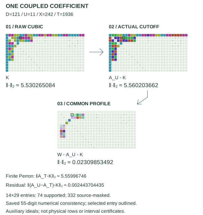 Original figure TeX · Source-matched figure PDF
These proofs use de Faveri’s pinned arXiv:2610.04045v1, Theorem 1.1 and its stated character family as external input. The primitive Poisson convention agrees with its Lemma 3.1; the formulas below also derive the normalization. This is not a proof of that deep large-sieve theorem. The source version and independent proof reviews are bound by the accompanying source map; full third-party reading caches are not public source dependencies.
For use the primitive additive pairing Let be primitive modulo , extended by zero at nonunits of this actual conductor. For every , (40.140) At a unit this is change of variable. At a nonunit frequency the additive character factors through a proper conductor quotient. Primitivity supplies a unit in the kernel of unit reduction on which is nontrivial. Multiplication by that unit leaves the additive factor unchanged and forces the sum to vanish. Unit reduction is surjective prime by prime and hence by CRT. Parseval for this nondegenerate finite additive pairing gives For the unit conductor use its one-element convention . For coprime , the two CRT frequencies are and , so (40.141) The product is primitive because each ramified local conductor occurs in only one factor.
Here are the archimedean factors that a raw Gauss sum alone would miss. Put and With Euclidean Fourier transform , differentiating the two-dimensional Gaussian gives (40.142) Holomorphic or antiholomorphic harmonicity removes the lower contraction terms. The sign is for either sign of . Let and . Its theta series is The lattice has covolume and dual lattice . Write a dual point as . Then and . Equations (40.140) and (40.142), applied in each residue class, yield (40.143) The inverse different and the conductor generator have not been replaced by a raw character value at .
Use and Every nonzero ideal has six generators; their contributions agree because . The Mellin transform of the theta series, with exponent , is therefore exactly . The same constant occurs on the conjugate side. Mellin integration of (40.143) proves the root formula for . At nonunit conductor the zero frequency vanishes by primitivity. At unit conductor and , . At unit conductor and , retain the Gaussian zero term when splitting its Mellin integral at one; this gives the usual meromorphic polar terms and root one. They are not dropped from the functional equation.
Changing to multiplies its Gauss sum by and its angular factor by , whose product is one. Thus the formula is independent of the conductor generator. Complex conjugation gives , where ; together with the angular factor this proves . Finally This proves (40.121) also for radial unitary twists.
In (40.141), the angular cross factors convert the finite residue values into ideal values . The remaining factor is . Radial cross factors satisfy Iteration proves (40.122). Coprimality is a hypothesis on the actual primitive ideal conductors, not on rational norms or higher induced moduli.
Let the types of be . The character in (40.120) has types . The three primitive conductors are pairwise coprime; no good local ramification can cancel against the other two. Applying (40.122) gives (40.144) Source reciprocity is . Substituting in (40.144) cancels all crossed values and proves (40.123), with . In particular the remaining factor is , not an assumed class constant; need not factor through the source class group.
For good dual , write , with the fixed finite reciprocity phase in that class. Then (40.145) The equality includes raw collision zeros. This is a fixed unitary row phase for each component, not equality of the two column classes. At the separate scalar is kept, including zero. There is no division by such a scalar, and no substitution of at a conductor drop. Off the original coprime column support, products of individual column gauges below are only an auxiliary extension. They are not roots or primitive conductors of overlapping pairs.
The endpoints in (40.124) are integers. The two smooth transitions lie between ideal norm nodes, so its value at is exactly one or zero according to the original interval and capacity. For nonempty fibres these transitions are disjoint. Their monotonicity gives total variation two; their th derivatives cost powers of . The elementary identity (40.146) follows by expanding the squarefree indicator and then the remaining coprimality indicator. Auxiliary need not be squarefree, and may overlap or . The original norm support fixes and before Poisson. Including more would add zero primal terms whose individual dual windows need not be zero.
On good , expand exactly This includes every reciprocity/ray component, not a selected same class term. With , good- deletion is the finite identity (40.147) Primitive zeros at suppress the corresponding terms automatically. They do not assign forbidden raw values to an original row.
For a nonprincipal primitive type-zero of conductor norm , its normalized functional equation and ordinary Mellin inversion give (40.148) To see the field constant explicitly, put The Mellin transform of (40.125) is . The Bessel identity may first be justified absolutely in ; smooth compact support and repeated Hankel integration by parts continue it to at each fixed . Mellin inversion of the primal ideal sum, its primitive functional equation, and the change now give (40.148) with exactly . There is no principal residue since has nonempty good ramification. The intermediate contour moves involve the entire nonprincipal completed function and the fixed smooth transform, not an inverse function or an assumed zero-free strip. This also recovers the pinned source Lemma 3.1 convention.
At a good prime ideal of norm , a nontrivial primitive character modulo lifted to , , has raw Gauss sum zero for a primitive additive frequency. More generally it vanishes unless the frequency has valuation , when its value is with compatible additive normalizations. This follows by summing the lifts first. Thus neither lower character order nor a higher physical modulus licenses a unit root. Applying (40.148) only at the actual in (40.120), and inserting (40.147) into (40.146), proves the exact signed kernel. Splitting every dual ideal uniquely as , with supported on and good, retains all modes.
The external sixth-order norm gives the following arbitrary-column- coefficient comparison, for every : (40.149) For completeness, extract with sixth-power-free . Freeze as the original column collision mask and apply (40.109) to . The four sums have factors , the count , and , respectively. Ideal counting proves (40.149). This is not an arbitrary row-weight theorem or an extension of a residue-subtracted energy estimate. For use the direct unit residual column; below there is no annular residual column. Primitive is not treated as sixth-order: convert to raw inside each fixed residual-class positive norm, where its common row phase cancels.
At , use (40.123) to form the two distinct vectors (40.150) The pairing is , not a PSD form at . The exact remaining primitive-conductor factor is (40.151) with scalar and finite weight . Its exponent is , not its inverse. On its modulus is at most one.
Insert exact gcd inversion before comparison and put , . Residual may overlap each other but are individually coprime to . Raw multiplicativity gives Their source classes are and , generally different. Bilinear Cauchy in the row variable, including (40.145), gives two separate positive norms. Only inside them may the raw mask be dropped. Uniformly in the fixed column phases and , (40.152) Indeed and an annular subsequence has columns. Neither nor is factored. For the small residual interval the direct unit count has the same bound.
Apply (40.149) to the two separate vectors. The divisor sums have exponents : (40.153) with the direct endpoint understood. For , the weight modulus is at most and the legal positive row prefix is . The four positive row exponents in give This is a summation over all -supported modes, not an exponent-zero convergent sum or a missing raw value.
The sharp requires an honest transform bound. Integration by parts against its finite variation gives For fixed , Stirling’s ratio estimate is . Thus (40.154) using the integrable tail and . No derivative seminorm growing with is hidden here. Only after the joint estimate may the original finite sum be bounded by ; the identity has not been Euler-completed. Finite , the original divisor sum, and unweighted actual counting cost a fixed constant and . Equations (40.152)– (40.154) give (40.155) Every finite source/ray component is reconstructed using the distinct gauges and bilinear argument, rather than a same-class inference.
For , each of the four powers of after multiplication by is positive. Finite dyadic summation, a last partial band and the dual unit separately therefore give the same bound with for every finite prefix . For a requested final loss , fix , independently of all scales, and use the positive-norm loss . Since , This proves (40.128); neither endpoint nor is invoked.
For the independent all-orders bound, expand exactly at every finite dual prefix. The th moment satisfies . The resulting original-column factors and are contractions, including on ; they are not replaced by . The exact factor is , and the finite norm exponent is with the same character phase as before. After gcd inversion, weighted bilinear Cauchy may bound inside each positive norm; the product of the square roots costs , not . All remaining divisor//subsequence constants are uniform in . The th joint bound is the prefactor of (40.129) times . Summing this absolutely convergent series proves (40.129) without an infinite-dual interchange.
For completeness, the scoped critical-half estimate uses . Its Fourier transform is . The fixed smooth step and its two transitions give and . The minimum of the three Fourier bounds , and has integral . On the half line exactly. The original finite square-divisor sum is harmonic, ; it is not an infinite . The same joint argument in the stated same-class/ component proves (40.130). This estimate is not summed over all dual bands to infer a whole target.
For define Fourier inversion of gives its full vertical limit . Integration by parts in each oscillatory tail gives (40.156) There is no pole-free inverse- contour assertion. Set . Every divisor norm is a positive integer, so The indicator is exactly , even when is an integer. Since , (40.156) is at most . A product of the two indicators therefore has error at most .
For squarefree put There are exactly ordered disjoint divisor assignments. On the supported coprime products only, , so (40.157) Forbidden entries of remain zero. The integral is the actual operator , with an ordinary right diagonal, not a Hermitian assumption. The two diagonal norms cost , , and each normalized absolute vertical integral is .
A uniform entry error alone does not multiply operator norms. Instead, with counting norms, The accepted fixed-field ideal bound gives an error at most , less than the displayed constant. This proves (40.131). Splitting the finite set of prime ideals from the rest proves . Use and to obtain the subpower/log bound. This is a mathematical finite-matrix transfer, not a claim of fast numerical Perron evaluation at that height.
Let . Two integrations by parts give . Split at to get Here and its support has length , proving (40.132). Absolute Fourier inversion expresses as an integral of two unitary norm diagonals and a scalar. Its Schur multiplier norm is at most . Compose with (40.157); two coefficient occurrences cost the square. All original zeros remain throughout, and no factorization of a primitive is supplied by this lemma.
Fix the scope of Proposition 40.24. On good arguments the primary-generator source construction is index-multiplicative. For , comparison with the unit source class removes the conductor of ; its type is zero. For and , The primitive conductors are coprime and their angular correction in (40.122) is one. Multiplication by the actual yields Source reciprocity is , proving (40.134). In the product for residuals , their common and cancel: (40.158) If , the primitive cubic conductor is , nonprincipal when . The same source class cancels its component. Common good primes have dropped only from that primitive conductor; the full union still remains excluded from .
The other common phases from and the modulations cancel in the pair. Their raw zeros, together with the factor, retain This notation means coprimality with the union of the displayed prime supports. Primitive values at are legitimate unitary phases of a good-conductor character. The radial factor is kept, not called a cancelled phase.
At fixed the core matrix is (40.159) Its cubic character already has the zero. All additional fixed residual phases are column contractions. On good arguments the squared sextic symbol is the actual primary cubic symbol . The pinned external Example 2.2 constructs precisely this family with primary generators congruent to one modulo . Both variables are squarefree and hence cube-free; source-sixth-class selectors and deleting the prime above only restrict the positive matrix. Theorem 1.1 at , or its transpose, therefore gives (40.160) The lengths are physical ideal norms , not varying conductor labels.
The original annular condition implies , a bounded number of dyads with lower endpoint at least one. On the encompassing rectangle , apply Proposition 40.23 with . This is the necessary repair: depends on both matrix indices and cannot be put into a fixed coefficient vector by fiat. Composing the common costs . With , the squared row radial factor is , and the column squared norm is The product is . Thus the two Mellin vectors have squared norms at most Cauchy in now uses , explicitly losing rather than exploiting its sign. A final triangle over gives the new inner branch (40.161) The accepted separate positive-divisor argument gives : there are divisors and each actual subsequence norm is . Both estimates apply to the same quantity, so their minimum is legal.
For , put . The new branch uses the convergent positive exponent-one sum ; the old branch uses its four positive exponents. Sum each branch to obtain the minimum after summation. The same finite majorant, bounds, actual count and fixed-line BV integral as above now prove (40.133), including the once-only normalization. No all-divisor or whole-dual conclusion follows.
On rough prime divisors , , no short divisor can contain , so exactly. The remaining fixed-residual arithmetic sum has the shape (40.162) up to the already fixed residual phases, with . Here is constant. A fixed-field scalar Mertens estimate is not a uniform bound for these varying cubic prime twists. The auxiliary principal case may cancel against other divisor sectors; it is no physical lower obstruction.
Factor the common rational norm prime by prime. At an inert prime there is only one ideal of norm ; equal norms force the same squarefree valuation in both columns and coprimality forces it to zero. The same argument excludes a ramified prime. At a split prime write the two pairs of valuations as . Then and . Sum two is forbidden; sum one forces opposite choices. Hence and the common norm is rational-squarefree supported on split primes. Both primes above each such prime must already be good. This does not assume that the original is conjugation-stable or enlarge it. Each eligible has exactly one partner, so the ordered pair count is at most . All other rational-nonsquarefree norms remain in the full annulus; only this sector has been classified.
The ternary bound is uniform in the original cutoff: . For each actual row the absolute triangle in this sparse sector costs before normalization. Divide once by and sum the actual rows to obtain (40.135). Original row masks give , and a nonempty capacity block has , hence . For each fixed , proves the target equivalence stated in the core, with constants allowed to depend on that fixed profile.
Conjugating the residue-field definition gives, including zeros, (40.163) For a split rational , exactly when meets at least one of its two conjugate primes, so the right side retains the original union zero. For an orientation of rational- squarefree norm , restriction to rational integers gives a primitive Dirichlet character : is an isomorphism, and each local character has exact order six. Its ideal norm pullback has conductor and infinity type zero. There is no smaller radical or common truncated-frequency assertion.
Choose one prime above each admissible split rational . Every divisor of an orientation has a unique rational divisor norm and the same Möbius parity. Thus with the two original cutoffs, and the partner has the same coefficient. At , (40.163) makes the local orientation factors and its conjugate. Expanding their product gives all ordered orientations exactly, proving (40.136). Both reversals are included, not divided by two. The common complex profile gives . For and no raw collision the character factors are , so they need not vanish or be positive; or can still vanish. This is not a row-energy lower bound.
For (40.137), use the exact primitive representation restricted first to these pairs. Its conductor norm is , and by on real . The Poisson amplitude is at most . There are integral dual ideals in a prefix or band, counting every -supported ideal once. The finite square-divisor sum is bounded by its convergent positive majorant; finite /ray and divisor costs give . With the sparse pair count and coefficient product , the numerator is . Division by proves the bound. This uses no general row-weight norm and no root cancellation.
At fixed parameters, exact Poisson gives , with its actual smooth derivative constants. Therefore (40.164) This is a signed whole-minus-prefix identity and triangle, not absolute summation of high modes. The condition gives pure and mixed target-sized prefix/complement sectors. Unequal norms and arbitrary larger individual windows remain unestimated.
This last construction concerns the pure block only. The primary section on good ideals is multiplicative because is bijective. Let be fixed, -supported and divisible by , large enough for all actual row-ray congruences. For coprime to it, put Every good local factor is nontrivial sextic, so its finite conductor is exactly , including nonunit frequency zeros. It need not yet be unit-trivial or an ideal character. The finite indicator imposes residual generator , original -goodness and the actual ray condition on . It is independent of . Literal square-divisor inversion is (40.165) The original zero is kept. Auxiliary lattice need not generate a squarefree ideal.
Use the same positive additive-pairing sign as above. CRT separates the common-modulus Fourier transform into the sum at frequency and the sum at . Primitive finite Gauss Fourier proves (40.138) for every , including its zero at . This is the finite recombination of all ray components; it is not a unit root at the larger induced modulus . For the Euclidean radial transform is At the common dual vector this equals . The lattice covolume is . Consequently, writing , (40.166) No class/root phase is discarded: the original finite function itself has been transformed. Primitive-conductor descriptions induced to the common modulus must reproduce precisely this frequency support, rather than a falsely flat lifted Gauss sum.
Combining the formulas gives the explicit signed literal additive band (40.167) All finite , the original unfactored coefficients and the full pair/ray/raw masks precede any absolute norm. There is no gcd triangle or positive completion in this identity. The frequency band is literal and unit-invariant; it is not simply the old primitive-ideal band under a new name.
On , the fixed-residue Fourier frequency is zero. The factor cancels and This -local mean is not the global , which is zero by primitive nontriviality. A six-unit orbit sum in this radial band vanishes if is nontrivial. Otherwise it is six times the sum over all integral ideals; values there are defined with any generator, not a nonexistent primary generator for an -supported ideal. At , local residue powers give Every good prime-ideal norm is one modulo six, and , proving (40.139). In the surviving case is a primitive type-zero ideal character and . The exact retained mean channel is (40.168) This includes nonunit and -supported dual modes. The phase is cubic, , not one, and its original cutoff has not been Euler-completed.
For the basic above and no additional ray condition, modulo the allowed coordinates are . The fourth primary residue is excluded by the original -adic coprimality condition. Thus , , and exactly. Dropping that condition would give the incorrect . The new exact local Fourier check has ; it is a finite -ring consistency check, not an arithmetic-family or asymptotic band test.
Proposition 40.25 controls the whole primal equal-norm sector. That alone does not control this sector in an individual literal band or -mean channel. To formulate a literal unequal-norm problem, impose on the original pair sum before applying (40.165) and (40.166). The projected formula retains unequal norms congruent modulo as well as all complementary literal residues. Neither the full nor its separately projected unequal-norm version is proved small here. At a pure critical block a sufficient band estimate would be with the fixed-profile dependence retained. This is not necessary for the whole kernel, where bands may cancel. Finite ray/root recombination alone does not provide it; nor does a nonzero local mean give a lower bound for the whole band. This identifies the remaining coherent unequal-norm arithmetic problem without deleting its means or changing any original conductor, capacity or profile.
Shared TeX sources: gauss-tail-core.tex · gauss-tail-figure.tex · gauss-tail-details.tex
The coherent kernel of Section 40.29 contains a difficult root-weighted mean. A large part of its short-divisor expansion can now be bounded by retaining a cubic interaction before taking a triangle. This gives a signed cutoff comparison, not a smaller norm for the original coefficients. A direct exact-discrete-frequency version is included as well. The remaining small-short-divisor moment and the separate discrete-frequency error are stated below. The whole signed power and global unsigned power do not change.
Keep , , , and the fixed exclusions of Section 40.29.1. A good ideal is prime to . All columns are the complete good squarefree ideal annulus , . Equal norms do not identify ideals. For a real cutoff put (40.169) Here is the original fixed unitary finite-order character; is the fixed literal unit/-supported factor with no good support. The actual coefficient is , . The function is one fixed, possibly complex, smooth common profile supported on , zero at the endpoints. Define (40.170) This explicit seminorm is finite and controls . It is a seminorm of the column profile, not of the sharp nodal row function.
Only the original unweighted pure two-pivot block is used: , , and the other four factors are units. The first row is good and squarefree, with the original literal/ray conditions and capacity. Its integer endpoints are (40.171) An empty interval contributes zero throughout. Otherwise . Use the exact of (40.124), its transform in (40.125), and . In particular , , and . The original pre- cutoff is never recomputed after another deletion.
Let be the original ordered coprime column pairs. One may also impose the original unequal-norm projection; the same choice is then used in every expression below. For each source pair and original ray character use the primitive , and of (40.120). Thus , and has total infinity type zero. Put (40.172) The symbol means avoidance of every prime in that set. Squaring never restores a deleted prime. Values at and at any later -supported frequency are separate primitive values, including zero.
In the exact primitive kernel (40.126), write each dual ideal uniquely as : is -supported, is good and sixth-free, and is good. Overlap of is allowed. For set (40.173) The top band is , . Replacing its count by its principal fixed-ray density defines the retained mean . This operation keeps, rather than deletes, its coherent main term. The selected branches are . At this top window , so runs over all integral ideals of norm below , including -supported ideals.
Set (40.174) On original coprime support the density is . For in the preceding sets, with , define (40.175) The exact definition of the normalized retained mean is (40.176) All sums here are finite. In particular there is no or condition. The finite original source/ray coefficients have not been centered. An argument at is not divided by a value at .
Put and define (40.177) Replacing both column functions here is an explicitly defined auxiliary model, not a change to the original primal data.
Proposition 40.27 (Matched leading model with its original cutoff). For the actual coefficients and every finite , (40.178) The constant uses no derivative bound for the sharp . Both interval endpoints and the original finite occur in . This estimates the model error, not the leading signed model.
For each good ideal use its primary generator and write for its positive residue character of order . For good squarefree put (40.179) The second expression is the normalized finite Gauss sum at frequency , including zero when . For put . Let be the actual finite part of the total type-zero , at its own primitive conductor . Then (40.180) The unit-conductor convention is one. This scalar has modulus one; it is not obtained by discarding the infinity type of a constituent. The accepted Jacobi character in (40.33) gives , with conductor of norm and nonzero infinity type. The exact root formula is (40.181) No extra quadratic sign is inserted. In the original kernel, and the second-row phase, when present, produce the raw cubic frequency ; here . This incomplete weighted frequency set is not a complete residue average.
For squarefree there is an exact sign-preserving assignment identity: (40.182) The factors are pairwise coprime and squarefree. For the difference of cutoff boxes has two disjoint pieces. After interchanging in the second and setting , the exact coefficient is (40.183) It is independent of . The conjugate Gauss CRT identity retains the cross interaction (40.184) The raw cubic entry is zero at a common prime.
The deep input is explicitly external: de Faveri, arXiv:2610.04045v1, Theorem 1.1 and Example 2.2, at . For the physical primary cubic matrix on good squarefree ideals of norms comparable to it gives (40.185) Both indices are actual ideals and hence cube-free, not arbitrary primitive-conductor labels. This is the same pinned input as the cubic comparison in Proposition 40.24.
Theorem 40.28 (Actual Gauss-weighted cutoff tail). For any bounded multiplicative ideal function on good ideals, with , and , (40.186) The constant is uniform in the conductor or raw deletion set in . For the actual pure leading model, with every original finite , class/ray/root/ component and coprime pair retained, (40.187) The original unequal-norm projection is also allowed.
This uses the cubic interaction before the short-divisor triangle. It does not assert pointwise or coefficient-norm shrinkage of , nor a separate cancellation theorem for .
Combining Proposition 40.27 and Theorem 40.28 gives (40.188) At , and , the errors are target-sized. If the coefficient tail is exactly zero; otherwise the three displayed powers are , and . The remaining exact coefficients satisfy (40.189) The small-short-divisor, long residual-Möbius cubic Gauss bilinear moment is still unestimated at the target.
There is also a direct reduction that does not introduce the principal-density split. Its exact support is (40.190) There is no squarefree restriction on . Overlap of and of remains allowed. Let be the same outer set as above, but with every original , and put (40.191) This is an explicit definition, not division by a density or a primitive value. With the original support as in (40.172), define the normalized exact piece (40.192) Then is the actual original top primitive-prefix contribution divided by . It is a signed representation-fixed piece, not a positive energy or the whole infinite dual sum.
Let be exactly (40.192) with replaced by . Only in that leading model can the finite sum be factored as . The discrete sum and its endpoints remain. Unlike , this model has no density, no projection and no integral replacing the family.
Proposition 40.29 (Direct original-prefix cutoff reduction). Put . With precisely the original support, (40.193) and (40.194) In particular the actual original piece satisfies (40.195) The original unequal-norm projection is allowed.
At the critical pure parameters used above the three powers are again , and , with exact zero coefficient tail when . This is a reduction of the actual discrete piece to a different, still unestimated, small-short-divisor model. That model retains every , every nonunit mode, the exact support, root/conductor data, original finite and both long residual-Möbius column coefficients.
The accepted fixed-ray disk count gives the distinct top-band certificate (40.196) Its pure critical power is ; this is an upper certificate, not a lower bound for the actual error. The direct reduction in Proposition 40.29 does not introduce that split: its discrete model retains those effects. No improved bound for the separate discrepancy, for the remaining small-cutoff models, or for the other original sectors is proved here. The result is an application of a named external cubic sieve to an actual arithmetic tail, not a new sieve, a complete analytic Lean formalization, a determinant/zero-location bridge or a proof of GRH. Fixed-profile constants and the explicit cannot be replaced by a uniform supnorm-only claim for varying profiles.
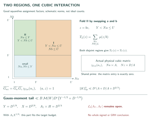 Original figure TeX · Source-matched figure PDF
The arithmetic norm input is the explicitly pinned de Faveri, arXiv:2610.04045v1, Theorem 1.1 and Example 2.2, at order three. It is used on its actual primary cube-free ideal family. We do not reprove that deep theorem. The primitive root conventions are those already established in Proposition 40.20, and the Jacobi orientation is that of (40.33). The accompanying source map binds the accepted research proofs and their independent reviews. Full third-party reading caches are not public proof inputs.
For a good ideal , the original fixed-source transport in (40.120) gives (40.197) This is an assertion about the total character on good arguments, not about the order of the individual possibly angular/radial . Write , and let be one if it is principal on good ideals and zero otherwise. The conductor of belongs to fixed data.
Here is the fixed-ray counting input, with its full deletion. For , the classical disk estimate gives (40.198) We recall a proof to specify the uniformity being used. For a fixed ideal modulus, count elements in each translated lattice coset inside a disk of radius . Convolve the disk indicator with a fixed compact smooth nonnegative mollifier of radius . The smoothed disks of radii and sandwich the original disk. Their zero modes differ from its area by .
For a nonzero dual vector , polar integration gives (40.199) The decay follows directly from the angular integral for : for , remove arcs of length around the two stationary points. Their total contribution is . On the complement integrate once by parts in the phase; the boundary terms and the integral of the derivative of the reciprocal phase derivative are also . For the angular formula gives the bounded estimate. Thus no unproved cancellation of lattice points is inserted. The mollifier supplies arbitrarily rapid decay beyond . Counting points of the fixed dual lattice in unit-width radial shells yields (40.200) The translation only changes unit phases. Choose comparable to for large . The boundary and dual errors are both . Bounded is absorbed into the fixed constant.
A type-zero finite ray character is a fixed periodic generator function, trivial on the six units. Apply the preceding count to its finitely many residue cosets, and only then form the possibly complex weighted sum. Division by six and the covolume of give the coefficient . The principal coset average is the good- density; a nonprincipal character has mean zero. For this proves the undeleted error . For the ideal count is zero and , so the same ideal estimate remains valid; is exact.
Now use the entire finite inclusion–exclusion: (40.201) Divisors with are still present, with their subunit arguments. For principal the main sum is ; otherwise it is zero. The error in (40.198) follows. Its final divisor product is by separating finitely many small primes and using at all sufficiently large . This is ideal-squarefreeness, not rational-squarefreeness.
For fixed , the original sum over has weight . In the pure block the scale is (40.202) Closed prefixes at both endpoints give the exact error formula (40.203) There are no half-weights at ideal norm ties. The angular representations of imply, with , (40.204) Indeed and ; differentiating the Bessel factor, not , proves the last assertion. Consequently the error at each fixed outer set is .
At the top window . Every good ideal of norm below is sixth-free, because a nontrivial good prime has norm at least seven. Therefore the unique decomposition into its part and good part runs exactly over all in (40.176). The principal condition is precisely . On the original coprime support . This proves the stated finite formula for .
For the separate error, , and there are original annular ideals. After normalizing once by , cancels the two column counts. The /ray/ sets are fixed, the top set is finite, and the original finite sum is majorized by . Since , this proves (40.196). Only its error uses these triangles; the mean in (40.176) stays signed.
The finite cubic sum at frequency is (40.205) For a unit frequency this is change of variable. At a collision, one local additive frequency is zero and its nonprincipal local cubic character has zero sum. CRT proves the assertion for every good squarefree ideal, including inert primes and nonsquarefree rational norms. The normalized sum has modulus one at unit frequencies.
The total has type zero, so the previously proved root formula is its finite Gauss sum divided by . CRT at the coprime primitive conductors gives exactly (40.180) times . Although their product is unit-trivial, the finite and good- characters need not be unit-trivial separately. No extra unit average is taken. The actual finite character, including its conductor drop, is used at its own primitive modulus. At unit conductor its Gauss sum is one.
On good squarefree , all local powers are nonprincipal and primitive. The Gauss–Jacobi identity therefore gives (40.206) Over a residue field this follows by setting in the product of Gauss sums; the zero- term vanishes because the product character is nonprincipal. Multiplication by CRT proves the composite identity: its additive cross multipliers on the left combine to those of on the right. The Jacobi sum itself has no additive-generator multiplier.
The correctly oriented result already proved in Section 40.19 is (40.207) Its sign is fixed by and for the positive sextic character. The reduction argument includes inert primes. Unique generators congruent to one modulo then identify with . Multiplication yields the displayed identity only on squarefree columns. In particular has its actual infinity type ; it is not a finite-order gauge.
Cubic reciprocity for the same primary section and the fact that yield (40.208) The cubic cross factors cancel, while . The quadratic Gaussian evaluation in the same two-factor completion is , with the period-four formula in (40.181). For composite , this uses that Gauss evaluation with its exact pairing; is not the root-count function of a composite residue ring. Combining these facts with (40.206) proves (40.181). There is no additional factor.
For the original good , (40.209) Before the pure specialization the row factor makes . All raw collisions are zeros. The separate original condition is not replaced by a frequency assertion. The primitive factors at and are and . When expressed with generators, their parts are the separate factors and . If either is zero the component vanishes. No quotient of these arguments, division by a primitive zero, or primary section for an -supported ideal is used. Changes of these generators cancel in the total unit-trivial character.
For and an integer , the angular cosine formula and its real Taylor remainder give (40.210) Indeed use the cosine Taylor polynomial through degree inside its angular integral. The remainder is at most , and the normalized angular moment of is . This proves both the coefficients and the bound for every nonnegative , without an exponential majorant or a sign assertion about the error.
Set (40.211) The exact order- signed model of (40.176) is (40.212) The character in every is still . Both finite endpoints, every primitive root and every original finite cutoff remain. In particular and (40.212) at is exactly (40.177).
Applying (40.210) before the original sum and the integral gives a per- bound (40.213) Only this certified remainder takes absolute values. On the full support . Since and is bounded by one constant independent of and all deletions, put . Counting the two actual annular column sets only in the error yields (40.214) Here the two column counts cancel , the /source/ray sets are fixed, the set has bounded size, and each interval has length at most . The constant in this inequality is independent of and of derivatives of . At it proves (40.178). The infinite Bessel hierarchy was already available; the statement used here is the finite real-axis certificate. It bounds the remainder, not the signed polynomial.
Freeze and one source/ray component in the pure model. After (40.181), every dependence apart from is a product of bounded multiplicative functions, except for two fixed finite selectors. The multiplicative factors include , fixed-numerator residue symbols at , the value , and the original deletion. They include zeros: a numerator valuation divisible by six does not restore a collision. Primary generators multiply on the required coprime products.
Let be the fixed source group and , of order . Finite character expansions give (40.215) The first coefficient mass is one. The second follows by normalized Parseval and Cauchy since the function has modulus one on . These bounds are independent of . Extending a fixed formula off its source class only extends a coefficient function; the finite selector sum restores the original class. No primitive root of a wrong-class or overlapping-conductor pair is asserted.
Consequently every actual fixed-other-column expression is a finite linear combination, of fixed total coefficient mass, of the linear forms in (40.186). The associated may have growing conductor and other-column deletion, but and multiplicativity on coprime products suffice. This does not flatten the original roots or make the coprime matrix positive. It is not a silent extension of a same-class, formula.
To prove (40.182), in each term of (40.169) set . Squarefreeness makes the factors pairwise coprime and . The cutoff difference is the exact disjoint assignment (40.216) Swap in the second piece and put in both. On coprime primary , Gauss CRT has the cross . Conjugation and cubic reciprocity give exactly (40.184). Thus the left side of (40.186), before taking its absolute value, is (40.217) At a common prime the cubic entry is zero. Hence this encompassing SF rectangle encodes the original squarefreeness of , without inventing a primitive overlapping root. Also , and the other fixed-numerator collision masks split in the same way. In particular the full other-column mask survives. There is no assumption that or is multiplicative. The elementary estimate is uniform in both cutoffs.
Use dyads in . Only , , can meet the original profile. Both indices in (40.217) are good squarefree ideals, hence cube-free. Primary cubic reciprocity identifies the entry with the physical family of (40.185), or its transpose. Additional row/column masks are coefficient contractions inside that arbitrary-coefficient norm. No character indexed only by a growing conductor is substituted.
Ideal counting and the divisor estimate show, with arbitrarily small exponent losses, (40.218) These are coefficient bounds after the exact signed grouping, not a new bound for the norm of .
The exact Mellin separation of the one common occurrence of is (40.219) Its powers are unitary on this line, so it costs once. The arbitrary-coefficient cubic operator norm and (40.218) therefore give (40.220) This is a bilinear matrix inequality, not positivity of the original coprime form. Summing the finite dyads with and gives (40.221) Dyadic logarithms and divisor losses are absorbed by distributing a prescribed among the preceding bounds. Partial dyads and real cutoff ties are literal coefficient indicators. Empty tails, including , are exactly zero. This proves (40.186).
Fix the other column . Its raw coprimality and numerator deletions are already in by Section 40.32.4. An optional condition is not multiplicative. The number of ideals of a fixed rational norm is at most the integer divisor function: at a split prime an exponent gives at most choices, at an inert prime at most one, and at a ramified prime one. Consequently there are ideals in the forbidden norm fibre, with all orientations separate. Since , subtracting it costs (40.222) This is below (40.186); by Fourier inversion. No whole equal-norm energy is subtracted from a different frequency sector.
The untouched original column has the elementary bound (40.223) Take this triangle only after (40.186). In the leading model all , source/ray and coefficient masses are fixed; is bounded independently of capacity derivatives, and supplies the two square-root norm weights already used. The normalization is once by . For each actual fixed , the column estimate is uniform in its bounded multiplicative numerator phase. Thus its original finite sum is bounded by , with no or altered conductor cost. One does not need to complete that sum.
Equivalently, define by . The preceding estimates give (40.224) For a tail on the second column, conjugate the scalar expression and reverse the roles. This sends to , to and the finite coefficients to their conjugates. The conjugate cubic matrix has the same norm, and . No Hermitian assertion about an individual source block is required. Finally use the exact bilinear identity (40.225) This proves (40.187) with all original finite cutoffs, primitive zeros and pair masks.
Equations (40.178) and (40.187) prove (40.188). When , substituting , , gives the exact exponent calculations (40.226) If choose ; the coefficient difference then vanishes identically, rather than replacing by a smaller number. The small-cutoff moment remains exactly the auxiliary expression with that . Since both short divisors have norms at most , their residual in (40.189) has norm at least . All other-column and finite-frequency couplings remain in its two-column sum.
The current separate discrepancy has critical power (40.227) This upper certificate is not a noncancellation theorem. A bound for the small-cutoff leading model alone does not cancel or improve it. Both it and the remaining original sectors require additional signed arithmetic.
For each original dual ideal, its good valuations determine uniquely with good and good part of sixth-free. At , the lower-open condition implies . Conversely every ideal of norm below has sixth-free good part, since the least good prime norm is seven. This proves the exact support (40.190) with all its nonunit modes and possible overlaps. No squarefreeness of or new coprimality with is introduced.
Equation (40.197) holds for every original . Retaining that factor and the actual discrete family in (40.126) gives (40.192). The prefactor is exactly , including the once-only normalization. All primitive factors at are still separate, and a good collision remains zero even when its exponent is a sixth power.
The pointwise real-axis remainder (40.210) at implies (40.228) Every argument in (40.192) is at most . Count only in this error: there are annular column pairs, , the original coefficient products are , and the original finite absolute budget is bounded by . The /source/ray and sets have fixed finite mass. Since , the exact good annulus contains ideals. This proves (40.193), without a ray count, interpolated endpoint, density or arbitrary row-weight norm.
It remains to justify applying the column-tail theorem to every original ray. The good- powers in the proof of (40.181) are local powers of ; that proof never uses . For every original component the total is type zero and its finite is fixed at its actual primitive conductor. Hence the finite selector expansion in (40.215) and its coefficient mass are valid on all these components. No new assertion of sixth order for an individual or replacement of a primitive Gauss sum is made.
Now freeze as well as . Relative to Section 40.32.4, the only new factor is . It is a bounded multiplicative ideal function and splits exactly in the grouped column as (40.229) The mask is a scalar which may be zero. The fixed phase is another bounded scalar. All earlier full-union raw deletions and separate primitive values remain. Thus (40.186) is uniform in as well as in , with no or cost. Their growing deleted primes are coefficient diagonals in the same physical cubic matrix.
There is no density in the new exact discrete model. Use the underlying arbitrary- theorem with the factor omitted, rather than dividing the earlier density-weighted moment by . If a domain has been written with deletion, first express it on the common original good-SF set with its exact raw zero. This permits a fixed column argument, restores no prime and adds no condition.
Apply the signed column estimate before the other column triangle. The latter is (40.223); after once-only it yields for each fixed and finite component, with the original factor. Sum the original finite norm weights and the fixed components. Only now use the count of the exact family. Reversed tails use conjugation, as in Section 40.32.7, and the original unequal-norm selector uses the same separate fixed-norm fibre bound (40.222). The exact identity (40.230) then proves (40.194). Combining it with the one Bessel error proves (40.195).
This direct proof does not assert a smaller value for the separate certificate in the continuous mean route; it never introduces that split. All of its nonprincipal-ray and exact-discrete effects remain in . At the residual column norms are at least , just as in (40.189). The new model is still unbounded at target size. It is different from the principal-density .
A capacity-empty integer interval, or empty exact , gives zero by definition. Absence of actual good squarefree rows in a nonempty integer interval alone does not imply that each dual prefix piece is zero; cancellation with other frequencies can be required. No full dual complement, other block, whole signed assembly or determinant/zero-location obligation is resolved by this direct small-cutoff reduction.
The inverse-different cubic Gauss frequency is incomplete: expanding it leaves the actual weighted primary set, not a complete residue system modulo . The bounded number of modes supplies no such completion. Likewise, expanding both short divisors and taking their absolute triangles before the cubic cross does not give the proved estimate. Even an explicitly hypothetical uniform inner exponent would produce the diagnostic (40.231) At this is . It is a conditional failure of that method, not an available smooth-coefficient Gauss theorem or an impossibility result. The actual proof above retains the physical cubic cross until its joint matrix norm. It bounds one specified signed tail and leaves the long residual-Möbius, finite- small-short moment as the next arithmetic problem. No whole signed, global unsigned, determinant, zero-location, analytic Lean or GRH conclusion is implied.
Shared TeX sources: ramified-gauss-core.tex · ramified-gauss-figure.tex · ramified-gauss-details.tex
The exact discrete prefix introduced in Section 40.31 can be estimated with its original coefficient . The argument constructs the previously missing finite-character transform at the ramified prime and groups all original short and Heath–Brown factors before taking a short-factor triangle. The resulting power is for this specified pure finite dual prefix. The whole signed comparison , the global unsigned comparison , and the remaining infinite-frequency assembly retain their earlier status.
The retained principal-density mean in the earlier discussion is a different expression with its own comparison problem. The result here uses every original ray component and the actual discrete sixth-part set. It supplies a new proof for the actual finite discrete prefix rather than modifying the historical cutoff stages.
Put , , and . A good ideal avoids the original fixed set , containing the primes above . All ideal columns are good and squarefree; different ideals of equal norm remain different columns. Use the unique multiplicative primary generator . The original character has fixed finite order, with its conductor exclusions in ; no order-dividing-six hypothesis is imposed on .
Assume (40.232) Only the original unweighted pure two-pivot block is asserted: , its second good factor and the other four good factors are units, and is the fixed literal unit/-supported factor with no good prime support. Keep its original capacity endpoints, nodal function , and pre- cutoff . An empty capacity interval gives zero. None of these data is recomputed during a coefficient decomposition.
Let be one fixed possibly complex smooth function supported on , with , and write (40.233) These are seminorms of the common column profile. No uniform derivative hypothesis on the sharp capacity interpolant is added. The exact frequency set is (40.234) There is no squarefreeness requirement on . The permitted overlaps among remain permitted, including nonunit -supported .
Here is a full definition of the piece being bounded. Let range over the original finite source/ray components and their ordered coprime good squarefree columns in , with the original source classes. An original unequal-norm projection may be imposed consistently. Use the actual primitive character of (40.120), its actual -conductor , and The numerator value includes its original raw zeros. Put . With , the normalized prefix is (40.235) All sums are finite. The ray label here is distinguished from the Jacobi column weight below. Values at and are separate primitive values, including zero; a conductor drop does not restore a deleted prime. The original occurs once. The raw numerator is .
Define by replacing in (40.235) by , with every other datum fixed. For the original coefficients the established real-axis estimate is (40.236) It uses , its fixed compact support and a pointwise Bessel remainder. The value may vanish and is never divided out.
The actual root calculation leaves one angular Jacobi gauge and a cubic Gauss root in each varying column. On good squarefree ideals the Jacobi function is , where has infinity type ; here is the chosen generator . The arithmetic belongs in the coefficient opening. There is exactly one varying , or its conjugate; an additional finite-order assertion about would be false.
Write for the positive cubic residue character, with its zero at every shared prime. The source Gauss root is (40.237) The actual root uses in this additive denominator. The normalization of the angular factor is explicit: (40.238) Thus the two fixed corrections may be written as source frequency . The factor belongs to the fixed finite character data; is not declared a good squarefree moving level.
After exact product-character expansion of the joint finite /source/ selectors, every remaining own-variable phase has the form , where belongs to a fixed finite residue family, with its original modulus-zero extension. It includes higher -primary conductors of . The finite source quotient is a fixed ray quotient; fixed numerator symbols are finite Kummer characters. The full Fourier sums retain their actual coefficient masses and reconstruct the primitive zeros. Growing other-column deletions remain literal masks.
For a physical good squarefree frequency , an exact interval , and a finite good deletion ideal , write the actual row in either required conjugate orientation as (40.239) Here is from this actual fixed family, including its angular factor. It is not an arbitrary bounded multiplicative function.
Theorem 40.30 (The actual fixed-family sharp row). For every such member, both conjugate orientations and every physical good squarefree , including the unit, (40.240) The constant may depend on the fixed conductor/character family. A literal unit calculation extends the estimate to ; for the row is zero with the stated endpoint convention.
Proof. Use the unconditional theta modularity and known integral cusps in Dunn–Radziwiłł, arXiv:2109.07463v3, Section 5 and Appendix A. Its weight-zero cubic theta is automorphic with Kubota multiplier on , where is the principal congruence subgroup of . Fix its known representatives and . The correct ramified coefficient projector acts on . Its primary selector is . A finite Fourier expansion writes it, and the away- periodic twist, as actual rational translates of theta.
For reduced, choose of determinant one, and choose so that . Use and . Then The multiplier is its literal Kubota value. Pure nonzero angular derivatives kill the pulled-back radial constants. Their Mellin identity has factor , including the Jacobian. The explicit cusp coefficients have absolute Dirichlet norm at most Normalized finite Fourier mass is and each reduced denominator has norm . This gives the conservative dual cost .
Coefficientwise cube completion retains the raw , with every stipulated Euler omission. Apply convexity to this entire completed numerator first. Its reciprocal is used only where , by absolutely convergent Euler products. Exact half-integer Perron thresholds and partial summation give (40.240). The optimized height is when this is at least one; the elementary count gives the other branch. The extended edition retains the constants and the zeroth-angular residues explicitly. ◻
On the actual contributing annulus , put (40.241) This is not the project’s original . Equation (40.241) is not asserted for arbitrary small columns or the unit. Unit factors inside an annular factorization remain present.
Theorem 40.31 (Original pure finite dual-prefix bound). Under (40.232), with the complete original support and fixed data of (40.235), (40.242) In particular its normalized leading power is (40.243) The raw numerator has one additional factor .
Proof. Open (40.241) and the exact finite Heath–Brown identity at . There are at most eleven factors, including the original . Choose their grouping from fixed independent dyadic scales. A balanced whole-factor partition has a physical cubic matrix bound , using the pinned de Faveri, arXiv:2610.04045v1, Theorem 1.1 and Example 2.2, at order three.
An unbalanced box has one long unrestricted coefficient-one factor . At neither an original short factor nor a short Möbius factor can occupy that scale. The product of all other factors has norm and its intrinsic signed assignment coefficient is divisor-bounded. This retains the boxes, which are all balanced.
For the cubic matrix gives . For , freeze the original opposite column first. Keep and all prefix zeros in its actual coefficient. The remaining long-variable deletion is . Its exact divisor changes frequency to and length to . Including the original prefix weight, Theorem 40.30 gives (40.244) Thus the small-prefix column costs . Choose ; both column costs have power .
Only after that bound take the opposite-column elementary count. Use the original once, sum the original finite with the convergent positive majorant , and count the exact family by . Optional unequal norms cost the same fixed-norm fibre bound . Finally (40.236) applies directly to . No -to- replacement or common-long-divisor opening is used. ◻
The estimate has fixed-conductor and explicit profile-seminorm dependence. It does not supply a supremum-norm estimate for varying , an arbitrary weighted-row operator, the infinite dual complement, mixed or neighboring blocks, short/principal assembly, an independent positive determinant, or a zero-location theorem. The Dirichlet, Hecke, Dedekind, elliptic and general Artin obligations remain separate. No analytic/category Lean formalization or GRH proof is claimed.
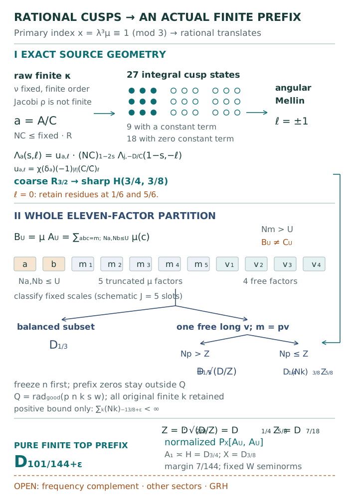 Original figure TeX · Source-matched figure PDF
The external theta input is the unconditional Section 5 and Appendix A of Dunn–Radziwiłł, Bias in cubic Gauss sums: Patterson’s conjecture, arXiv:2109.07463v3, 14 May 2024. Its GRH-conditional prime theorems are not used. The matrix input is the already admitted physical ideal family in de Faveri, Optimal large sieve for fixed order characters, arXiv:2610.04045v1, Theorem 1.1 and Example 2.2, at order three. The theta modularity and deep cubic norm remain external theorems. The constructions and estimates below specify how they apply to the actual finite-character family.
The full varying-column phase list, after the arithmetic opening, consists of one or its conjugate, the cubic Gauss root, the original finite-order , finite source/ray factors, the mod- Fourier factors of , the actual primitive -type factors, and residue symbols at the fixed numerators . The set , the -types and the set are fixed finite sets. The growing numerator belongs to the cubic frequency instead of this list.
There is a common fixed residue modulus for this list. A finite-order Hecke character has infinity type zero and factors through its actual conductor. The source group is explicitly a ray quotient: Section 2.3.2 of de Faveri defines for one sufficiently deep -supported ray modulus . The chosen primary generators realize these ray characters as finite residue characters. The factors are characters of .
The local sixth-power tests also have a fixed finite modulus. For a prime , Hensel’s criterion at gives when . One may use and . These are moduli for testing local classes, not replacements for primitive character evaluation moduli. For a fixed nonzero integral numerator , its -th residue function, , is a finite Kummer character for . A safe sextic conductor bound is supplied by the polynomial discriminant ideal . A field/order discriminant divides this separable polynomial discriminant, including when a proper factor supplies the field. A fractional numerator can be cleared by a fixed sixth power, retaining its original numerator and denominator exclusions. This uses finite one-dimensional Kummer characters, without a general Artin-holomorphy hypothesis.
A joint finite -type or primitive-value selector is not assumed multiplicative. If is its fixed finite residue group, write its actual function as (40.245) Normalized Parseval and Cauchy prove the last line. This expansion precedes freezing a primitive type or separating column factors. Forbidden primitive values are zero in ; individual Fourier terms can be nonzero there, and only their full sum reconstructs the zero. No term is individually renamed an original nonzero row.
Thus one may use a common fixed raw modulus and functions (40.246) They are imprimitive residue characters on that modulus. All stipulated prime zeros survive a primitive conductor drop.
The Jacobi function is not one of these finite characters. Its has already entered the arithmetic coefficient , and its unique remaining angular factor is , with order or in the two conjugate orientations. Common or prefix Jacobi factors stay in their actual outer coefficients when those variables are frozen. An arbitrary bounded multiplicative function, a growing opposite column, a Möbius coefficient or the nonperiodic density is not made into a member of this fixed family. That density does not occur in .
Let , and . The source theta function is a weight-zero function on hyperbolic three-space with for . The multiplier is the source Kubota character. The quotient has cosets. One can see the finite count from : the reduction kernel in has elements, and has .
Fix the published integral representatives and put . For the exact chosen function define its actual Fourier coefficient by (40.247) For those representatives for and zero for . The support lies in . The symbol always means this actual coefficient; a source table using , or a conjugated function is converted before using an exact phase formula.
The source formulas (5.7), (5.13), (5.14) and Appendix A express these coefficients through , unit rotations, fixed unit factors and additive phases. The first nine families have the absolute norm and the other eighteen have the norms. Rotations, conjugation and index reversal preserve absolute norm.
Proposition 40.32 (Known-cusp absolute norm). For , every one of these actual cusp families satisfies (40.248) The right side is independent of a moving good level or a translation. Here omits the prime above .
Proof. In the formula write , with squarefree and arbitrary, possibly sharing primes with . For the first family , , there are at most six sign/unit branches and For the second family , , there are at most two branches and . These follow from the literal unnormalized primitive Gauss magnitude and the source factor ; the fixed Gauss numerators are units modulo good . Retain the separate and cube variables. A generic coefficient bound would lose convergence near .
Put and , with the prime excluded. Then (40.249) The families each have three unit branches at , with magnitude at most ; their possible opposite signs do not change the norm. Consequently (40.250) In the stated range , , , and . The brace in (40.249) is at most . Finally . The actual coefficient convention and all unit phases therefore give (40.248). ◻
For later comparison, an affine state , , has index and coefficient (40.251) Its absolute Dirichlet norm is exactly . For the ramified diagonal , this factor is . Commuting a moving translation past that diagonal changes to . Together with its phase is still . This explains why an omitted ramified scale changes actual phases, even though the eventual absolute bound is fixed-data controlled.
For reduced, choose with and put . The Euclidean property of supplies this choice. Let Integral is included by . Direct multiplication proves (40.252) Choose with . Then the exact function identity is (40.253) It uses known integral cusp functions rather than an unconstructed new cusp coefficient family.
The phase is computable, not an unspecified unit set to one. Find a rational integral with the same reduction modulo as . Then . If , the source rule is (40.254) Here is nonzero and coprime to . The index can be found by reducing modulo and testing the -element rational subgroup against the fixed cosets. Equivalently, a finite traversal of elementary generators constructs representatives. A representative differing from the published one changes its function by the fixed multiplier just computed. Its Fourier coefficients and constants carry that multiplier too.
One can also display the fixed ramified states explicitly. If a moving good level survives the fixed denominator reduction, write , with in a fixed finite set and . The matrix identity and give the fixed state followed by the moving translation . The general formula (40.253) also handles cancelled or nonunit fixed Fourier residues directly; this special display does not impose a primitive Fourier-support condition on them.
Write . The action in (40.253) is (40.255) The pulled-back constant of is therefore (40.256) It is radial in . Every nonzero pure Wirtinger derivative or at kills it. At large the original translated theta constant is also independent of . The known nonconstant lattice support gives exponential decay after angular differentiation at both ends, with the reciprocal-end rate depending on .
For completeness, the zeroth-angular constants have not disappeared. For a finite combination put (40.257) Its regularized Mellin transform with weight has residues (40.258) These signs follow by integrating the powers at infinity and zero. A projector with zero sum kills , but need not kill . No finite noncubic label implies such a cancellation.
For set ; for use . The angular Mellin transform is (40.259) For it is entire by the endpoint bounds just proved.
Proposition 40.33 (Exact angular rational-cusp identity). For every reduced rational translate and , (40.260) The right Mellin transform uses the actual known function .
Proof. For , set in the full-coordinate chain rule. Then and in (40.255) are constant as functions of , while is affine with derivative . Thus the pure derivative has exactly the factor and the opposite angular derivative of at . There are no lower angular or radial terms. The negative sign case is the conjugate-coordinate calculation.
In the integral substitute . Its Jacobian and power weight give . Combining the factor produces precisely . The exponent , rather than , is essential. This proves (40.260) for both signs. ◻
If the real part of the dual Dirichlet variable exceeds one, its series is (40.261) The additive and angular phases remain literal; their absolute values are one only after this exact expression has been established. Proposition 40.32 controls the series.
Let be any one fixed residue member on the primary section. Use a fixed modulus containing its actual conductor and all original fixed exclusions. Separate its -part and away- part . Choose containing the -conductor, and put (40.262) The entire theta support has . The correct argument is this integral index, not for a ramified character.
From the two families above, selects exactly (40.263) Indeed the first family has positive -valuation after multiplication by , as do the second-family terms with . They are killed as nonunits. At the negative branch is modulo , and only the positive branch is . This proves the unit-state selection as well as its valuation condition.
For a moving good squarefree level , let be either cubic orientation on its literal residue modulus. Let be the fixed away- raw modulus. The product is a bounded periodic function on the valid period . This period is not asserted to be its primitive conductor. It is allowed to be imprimitive and to have overlapping . No value is divided out.
Define the coefficient-projected theta function using . Its infinite constant is zero. On , . Multiplicativity on the primary section gives the exact cube identity (40.264) Write (40.265) with every fixed raw zero in . Then initially , (40.266) The factor is the actual angle of . The cube series has denominator , and retains all original exclusions above , even after primitive conductor drop. There is no factor or untwisted-zeta substitution. Conjugating the whole construction gives the actual conjugate Gauss root and opposite angular/cubic orientations.
The full ramified projector has an exact finite translation formula. The trace dual of is , so (40.267) For the away period use normalized Fourier coefficients with positive inversion sign and pairing . Since avoids , that pairing is perfect, and (40.268) Both mass bounds are Parseval followed by Cauchy. They hold for arbitrary bounded periodic functions; no primitive Fourier-support condition is inserted.
Consequently the exact projected function is a finite sum of with (40.269) The inverse different explains the exponent . Every raw zero is reconstructed by this full sum. Each reduced denominator divides a fixed -power times ; hence . Nonunit Fourier residues may lower that denominator. They remain terms of the exact transform, rather than being discarded.
Let , and set For the finite sum of entire angular Mellins is entire. The source Fourier–Mellin calculation has factor (40.270) Thus division by , whose reciprocal is entire, and the nonzero elementary factor in (40.266) makes entire as well.
On , , (40.260), (40.248) and (40.269) give (40.271) The height exponent follows from the quotient of the two Gamma products. The exact multiplier has been written before bounding its modulus. This is a conservative cost. No refined Ramanujan estimate is used.
The line is absolutely bounded uniformly in , by the original Gauss and cube coefficients. For a requested final , choose sufficiently small in terms of ; the constants may depend on that choice. The finite-order continuation from the theta Mellin representation permits the damped strip maximum principle. Applying it to the entire numerator, then allocating small exponents, gives (40.272) on the safe half-strip . Only there divide by : the real part of exceeds one, so its inverse is bounded by absolutely convergent Euler products, uniformly in all raw omissions. No inverse- continuation through unknown zeros or zero-free strip is asserted. Equation (40.272) therefore bounds on that half-strip.
Here are the endpoint details needed for Theorem 40.30. Replace each real endpoint by the half-integer threshold selecting exactly the same integer norms. All ideals in a repeated norm fibre are counted. Such a fibre has divisor-bounded multiplicity in this quadratic field. For an unnormalized sharp prefix at length , truncated Perron at height has error (40.273) This follows by summing over integer distances from the half-integer endpoint . No norm tie receives a half-weight.
At the vertical contribution is bounded by If , choose . On horizontal sides the bound is at most , up to allocated subpowers, since . The vertical integral, truncation and horizontal contributions are then . An interval is a difference of two prefixes. If , the elementary count is the better branch.
Finally apply partial summation to the same , . Its supremum and total variation are bounded by . This proves (40.240) with the exact profile. For only the unit can occur; its coefficient and profile are literal and satisfy the same bound with a fixed endpoint constant. For there is no contribution. This extension uses no analytic theorem at a fictitious length.
The opened coefficient in (40.241) is asserted on the actual annulus . It is distinct from original . No identity for is needed or asserted. Unit factors within the factorization of an annular column are essential and stay in every convolution below.
Let be the constant-one function on good ideals, the ideal-convolution identity, and , . The exact good-ideal convolution identity is (40.274) Indeed , so expand ; also . Each factor of has norm strictly above . The last term in (40.274) is supported strictly above and vanishes at every residual under consideration.
The -th term has truncated Möbius factors and unrestricted coefficient-one factors. Together with the two original short factors it has labels. The term and unit labels remain. Restricting the total column to squarefree support forces all factors to be squarefree and pairwise coprime.
Use independent dyads , , with the original own-factor cutoffs at . If the box meets the annulus, (40.275) Choose the partition from these scales only. If some , it is a balanced subset. If all , multiply successive scales until first reaching ; the result is below . If no balanced subset exists, a unique scale exceeds ; two such scales would have product above . The product of all remaining scales is below .
At , Therefore an unbalanced unique long factor is genuinely one of the unrestricted coefficient-one factors. It cannot be an original short factor or a truncated Möbius factor. The actual whole prefix , the product of all remaining factors, satisfies . The term has no unrestricted factor and is automatically balanced; its unit assignments have not been discarded.
For a fixed box define each macro coefficient by summing all its signed assignments within its assigned factor group. On a squarefree ideal the number of at most eleven labelled factorizations is at most . Fixed binomial factors and dyadic logarithms thus give a uniform pointwise bound, with every own cutoff retained. There is no separate count over .
A balanced partition gives two physical squarefree macro ideals , each with scale in fixed multiples of and product comparable to . Their own coefficients contain the original cutoffs and signs. Cubic Gauss CRT gives on coprime products (40.276) The raw matrix entry is zero at a collision, so summing all squarefree macro pairs implements the original squarefree product. No primitive root at an overlapping product is invented.
The external physical cubic norm is (40.277) The rows and columns are actual good squarefree ideals. All raw fixed/growing multiplicative masks are coefficient diagonals in this norm, after finite-selector expansion. Ideal counting gives squared coefficient norms when each coefficient is weighted by the inverse square root norm. Separate the one occurrence of the common by The powers are unitary diagonals, costing once. Balanced boxes therefore cost .
For a Type-I box write , where has coefficient one and the intrinsic contains all remaining assignments. Then . The portion , with its literal own-variable indicator, has dyadic bound and hence total bound (40.278) Macro own-factor constraints remain coefficients. A chosen equivalent row-dependent norm interval costs the reviewed logarithmic interval-Schur factor, preserving complete norm fibres. It is not assigned operator norm one.
Freeze the original , the exact , and a finite source component before estimating a Type-I row. The original pair mask is exactly (40.279) The first factor stays in the actual prefix coefficient, along with all original prefix/ collisions, fixed numerator zeros and prefix phases. The intrinsic arithmetic still depends only on its own factor assignments. Multiplication by these outer factors preserves its divisor bound. A forbidden prefix is zero before a row bound is applied.
The remaining long-variable deletion is It is not a substitute for the first factor in (40.279), and the growing is not part of a fixed character conductor. On the nonzero support are squarefree and coprime, by the original zero. The physical cubic frequency is .
The exact deletion formula is (40.280) Insert and set . Gauss CRT and reciprocity combine the actual crosses into . This raw entry is zero at and encodes the squarefree-product condition. The outer raw entry kills . No zero is inverted, including if a numerator exponent becomes divisible by three. Original interval endpoints divide literally by .
Here , and the exact product is (40.281) There is no common-long-divisor decomposition between the two columns in this proof. The other original column remains fixed.
Using the sharp bound and the original prefix factor gives (40.244). For use the actual unit contribution; smaller arguments contribute zero, with the profile endpoint rule. Large frequencies are allowed by the proven all-level sharp bound, with its trivial fallback. Thus On the exact support, , , , so . Summing over by ideal counting proves the small-prefix column bound (40.282) Every prefix zero was retained until that positive estimate. No coherence or orientation mean has been removed.
Combine the balanced, large-prefix and small-prefix bounds, and put (40.283) The untouched original column has the elementary bound . Apply it after the left estimate and use the original once. All finite source/ray/primitive coefficient masses stay fixed, and the actual family is counted by only at the end. The scalar is bounded and is never divided out.
The original finite sum is unchanged in the identity. Its small-prefix positive majorant is (40.284) Product and divisor losses can be allocated smaller exponents first; their factors are absorbed by this convergent series. Balanced and large-prefix pieces use the easier exponent . This is a bound on a finite sum, not an Euler replacement of the model.
For the optional original unequal-norm projection, a fixed rational norm has ideal coordinates. The actual and every fixed HB component are divisor-bounded. Removing that same fixed- fibre costs in the left column, and therefore in the normalized form. Conjugate ideals remain different, and a norm inequality has not been made multiplicative.
This proves the leading-model part of (40.242). For the original exact prefix, all its Bessel arguments are at most , and There are annular column pairs and . The coefficient product is , the original finite absolute budget is bounded by , and the actual sixth-part band has ideals. Only in this remainder are these absolute counts taken. They give (40.236) directly for . No -to- error, principal density or scalar ray-count split is introduced.
Finally the exact powers are (40.285) The same norm-fibre correction has power . This completes the pure finite-prefix theorem with its once-only normalization and all original finite cutoffs.
The accepted evidence includes exact rational cusp matrices and finite quotient/coset calculations, angular-coordinate and Mellin checks, literal primary-support cases, affine coefficient transport, and synthetic scale-composition/exponent checks. The typed exponent grid is a formal subfamily; it is not exhaustive physical dyad coverage after the constants in (40.275). The proof uses the separate exact inequalities for those constants. None of these checks is actual-family energy data, training, asymptotics or a kernel-checked Lean proof.
All original sources, primary versions, raw outputs and failed preliminary harnesses remain preserved. The new theorem is a prose proof with the identified external theta and cubic-norm inputs. Its domain is the representation-fixed pure prefix in (40.235). The infinite dual complement, other pure sectors, mixed and neighboring blocks, short/principal assembly, independent positive arithmetic determinant and zero-location comparisons remain open. The Dirichlet, Hecke, Dedekind, elliptic and general Artin scopes retain their separate hypotheses; no Artin holomorphy, desired positivity, zero location or GRH premise has been inserted. The whole signed and global unsigned comparisons have not changed.
Shared TeX sources: paired-cutoff-core.tex · paired-cutoff-figure.tex · paired-cutoff-details.tex · wide-cutoff-core.tex · wide-cutoff-details.tex
The comparison in this section concerns a specified part of the signed coprime-column form for the original unweighted, nonprincipal, two-pivot Eisenstein rows. We use the physical ideal norms and the original ordered cutoff. Let be the column, cutoff and capacity parameters, with and . The first two row ideals have dyadic norms , , and the actual primitive conductor of row has norm . The finite bad-prime set , row type, and twist are fixed. The same smooth complex profile supported on is used on both sides. Ideal labels, including conjugate primes of the same norm, are retained individually.
For each good squarefree intermediate Möbius divisor , put . Let be its original row amplitude and the equal-norm part of the original middle Poisson window. We study selections of (40.286) Here the counting inner product is linear in the first argument. This is one term in the expansion of the original signed norm. In particular the intermediate is different from the gcd of the final column pair.
On an original allocation let with , let be the other deletion label, and put , with the original squarefree short divisor. Set The original middle window has and , for its specified . The primal test discards the guaranteed zero cells , and the original weights retain any further zeros. An allocation with belongs to the direct component. Its re-expressed Poisson sum stays in the complement in (40.286).
On the equality side write and , so . On the partner side the selected changes in the good exponents consist of erasing the squarefree cutoff part , erasing a part of the good conjugate overlap, and inserting allowed positive increments at other good primes outside . A conjugate erasure removes the full original exponent, which can be two. At an insertion prime the old residue plus the increment is at most five. Changes at the good primes of keep their exact new residues. For fixed other labels write and . The physical insertion ideal keeps each exponent and is disjoint from the selected erasure supports and . Thus and are physical lengths. The two varying raw phases are , or their conjugates if the pairing is conjugated. The fixed row factors retain the union of deleted primes, the literal section, the twist and the primitive -values.
The subtraction on the partner imposes only in its original middle window. At fixed this fixes at most one integer norm for , and the reverse count fixes at most one norm for . An integer norm supports at most divisor-many ideals on the polynomial clip. With the physical inverse , the paired count therefore costs up to subpowers. The two half radial powers leave The remaining harmonic weights give for this subtraction at each , with the inherited profile and subpower costs. Both original endpoints remain in the count. Equal norms in the direct and other components remain in the pairing.
The bounds have the common cost , where controls the indicated smooth profile derivatives. The live partner primal test supplies and partner radial scale . The proof first sums each actual column array. It then uses the row comparisons and the original label sums.
At the mixed scales , the selected normalized cross has upper power over all physical ratios and all . If , a perturbed primitive sharp moment gives the target power for the same selected cross on The second pivot need only satisfy the stated original admissibility and capacity. The conductor comparison uses the actual .
At the pure critical scales , , the target power holds over all in each of the following physical sectors:
, with any erasure length .
, with any insertion length .
and .
The flexible central windows give further short and long threshold curves. There are also separate comparisons for a small fixed residual label product and for a small -prefix. The comparable pure all-divisor comparison has power , and the target holds on in that sector. Each assertion concerns the selected changes described above. The remaining pure rectangles and the coherently averaged signed divisor sum are open.
Fix an ordered factorization of the actual squarefree cutoff label on either side, with and . Write . The assignment sum multiplying is Complete the -sum and then subtract its excluded terms. With in the subtraction, squarefreeness gives the exact identity (40.287) The complete -sum forces . The unit gives the indicator at , while the nonunit terms with vanish by the full inner Möbius sum. Both inequalities of the remaining band are strict. Below the product cap the band is empty. The three possible assignment values are according as both, just one, or neither individual capacity reaches .
Fix the row, both ordered factorizations and the primal and dual labels. Select both labels to be fixed -supported ideals, take the good changed-residue ideal on to be the unit, and require to avoid the full fixed prime union of the row and the primal and dual labels. When on both sides, their capacity step functions multiply the original outer Möbius sign. The fixed-field deleted Möbius estimate supplies subpower cancellation for the resulting fixed-label scalar on with for a fixed . In the pure comparable block, a physical -interval of width gives the target after the full divisor sum by a separate sparse erased-column estimate. This includes the narrow interval immediately above the product cap on the actual partner allocation. The wide correction and the remaining coherent signed estimate require additional arguments. The whole signed and unsigned powers and , the independent determinant comparison, and the scope-specific zero-location obligations remain as in the preceding sections.
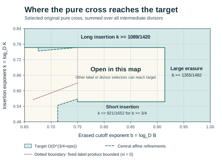 Figure generator · Source-matched figure PDF
Throughout this section, denotes the erased squarefree cutoff factor, the positive insertion ideal, and their respective physical dyadic lengths. The exact partner norms are and . Here is the original dual ideal, and is its fixed residual factor in a given cell. Write At the critical pure scales at the level of powers, and at the critical mixed scales . Fixed comparison constants in the scales are allowed throughout. A bound in this section includes the common factor for the paired cross, with the original fixed-data constants. In row moments the appropriate one-profile factor is understood separately.
The estimates concern the selected pairing with both original erasures, all positive off- increases whose sum with the old residue is at most five, and the exact new residues on . The old cutoff and conjugate erasures, including old exponent two in the conjugate erasure, remain in the phase. The cutoff is , with . The rows are the original unweighted literal nonprincipal rows. We keep the common , fixed , literal ray, capacity and squarefree selectors, and the actual primitive , Gauss root and raw zeros. The physical sieve is the order-six application in Section 40.28. Its exponent at column length , relative to , is (40.288) Its growth slope is at most one. A live subunit dyad is treated at constant scale.
First remove the negligible inherited tail . Its absolute estimate applies to each selection below. Fix the original allocation and dyad on the partner side. The compact logarithmic separation of the partner profile uses . Its weighted Fourier absolute integral, with the extra factor in log frequency , is bounded by a constant times at the actual dyadic profile scale . This follows by extending the profile on a fixed-width log interval and integrating by parts. The phase factors then separate on the erased array, insertion array and row. There is no condition on in this separation. Sharp subinterval partial summation removes the insertion norm twist with the erased array and every other row multiplier fixed.
For the original middle equality, the equation fixes at most one integer norm on either side given the other ideal. There are divisor-many ideals of each integer norm on the clipped support. This counts the entire insertion ideal, including its powerful part. The physical yields weighted mass . The two half radial powers supply , giving the factor . The remaining label sums give . Apply this subtraction only in the original middle window with its exact two endpoints. Equal norms in the re-expressed direct, low and far pieces remain there.
The original live primal test gives (40.289) For each side write for the original grouped square-divisor label and for its deletion norm. The good part of is a divisor of , and its other part is supported on . Write with . The three ideals are pairwise coprime and squarefree. The ideal is distinguished from the length exponent . On the equality side . For the good part of the conjugate define The good conjugate erasure support is a squarefree divisor of avoiding . Its full erased factor is . Let be the actual sixth-free new representative at the good primes of . With the original -part and the full sixth-power repetition, the exact partner residual is (40.290) The quotient follows from the good exponent difference of the two primitive phases. Away from , before changing any residue, that difference has representative exponent At one adds six to the negative exponent, and at one subtracts the overflow six. The selected cutoff erasure removes from this product. The selected conjugate erasure divides by , and the -part uses in place of the matched residue. The positive increases multiply this exact residual by . The norm and raw value of are retained, including any overlap with the other factors. On the original admissible pairs these operations give the literal product times the fixed row phases, with the original raw zeros.
Let be the product of the two row norms relative to , after the projectors and powerful sums. The full cutoff inverse norm is included in these norms. For the exact paired scalar, start with Up to the fixed dyadic constants its profile scales are The actual profile uses , the physical ideal norms and the original fixed -factors. Multiplying by gives the following weights before the relative row moment: (40.291) The scalar is accompanied by the retained decay from (40.289). Every absolute comparison follows the exact pairing with those labels.
In the harmonic -count the fixed pays to power one. A conjugate erasure prime uses a distinct . Its conjugate lies in exactly one of , paying a second inverse norm. In the old exponent-two case, the original pays a third inverse norm. Thus the resulting local exponents are at most and , respectively. When or its half power is needed, charge . This charge is disjoint from both conjugate charges since , its conjugates lie in , and . The other sums below are harmonic on polynomial support, convergent inverse-power sums, or fixed-divisor choices.
For , take . The harmonic comparison at each is (40.292) The two three-half choices give the comparisons with the corresponding retained decays. In the second choice . With , the cancels, the weights in have exponents , and the disjoint charge on pays its half power. The resulting comparison is (40.293) By the first inequality in (40.289), summing the costs on its live range. The two three-half choices on cost and , respectively.
The higher choice leaves in (40.291). The exact primal restriction gives Write the remaining numerator as and pay the first two factors by the preceding harmonic counts. The additional and give the harmonic comparison (40.294)
There is also a fixed-label selection for . For , the original eligibility excludes , , and at most one of contains . The exact residual has valuation four or five at this prime before adding the full sixth repetition. Thus . On , the joint count of is , by summing . Formula (40.291) then gives . This selection is sufficient when . The comparison uses the full residual ideal, with its -part and repetitions.
Write uniquely, where is squarefree and the nonzero valuations of are . We have . Fix at first. The common-prime projector for uses , with and the two raw values on . Require itself to satisfy the original fixed prime eligibility of , including , before stripping it. The residual avoids by its squarefreeness, along with the original forbidden union. Keep the original fixed -deletion on the erased array. After stripping , the squared erased mass is , including its actual . The insertion length is . A dyad has powerful ideals, by the unique representation with squarefree and the convergent . Overlap is allowed at exponent five. This pays the shortening in the product of the two moments.
For the sharp insertion bound at length , expand the fixed deletion and squarefree selectors in the order , where divides the full forbidden union and avoids that union. All Möbius signs and fixed raw factors are retained. At fixed the remaining sharp interval is an unweighted -interval after the exact partial summation. Its endpoints can be treated as sharp disk endpoints. Smooth a disk of norm length at radial width proportional to . The normalized shell row norm is bounded by a subpower times To see the additive term, split each ideal uniquely as with supported on and good sixth-free. At fixed , the shell contains divisor-many ideals per integer norm and has norm width . Apply the physical sieve to . The square roots of the width weights sum absolutely. The constant atoms sum over , giving up to subpowers. This also accounts for open or closed endpoints.
The smoothed primitive Poisson transform has the original and primitive Gauss root. On a dual dyad put . The disk transform is times the Fourier transform of the unit disk’s chord length at frequency comparable to . Integrating once by parts, separating the two endpoint intervals of width , and integrating by parts again on the interior gives . The endpoint derivative integral is ; the interior boundary and second derivative terms are before the second division by . The same argument with the chord length multiplied by bounds the frequency derivative, so its logarithmic derivative costs one power of . The convolution bump and its log derivative provide for arbitrarily large fixed . Consequently the cutoff log function and have bounds and , respectively. Splitting the Fourier integral at and applying Cauchy and Plancherel gives absolute log Fourier mass . Multiplying by yields The zero frequency is absent by nonprincipality. With when , the effective dual exponent is (40.295) The main shell term has row RMS . The additive term has the same bound whenever . The smoothed term has that bound if . Above the cutoff the arbitrary smoothing decay pays the degree-one growth of the sieve and the divisor subpowers. The ordinary estimate applies directly if .
In pure use for . For the convex function in (40.295) before truncation is at most by the endpoints. In mixed use for . The smoothing branch requires , and the same convex comparison gives . The additive term meets the stated criterion in both cases. The exact deletion -sum has divisor cost at fixed , the -sum is harmonic, and the -count pays the shortening above. The resulting sharp rectangle loss is . It uses the physical ratio even when and are unequal. The ordinary two-moment alternative has loss .
The coupled comparison keeps a sharper tail for at . Freeze , expand the remaining by , with , and fix the powered portion on . Set and group the insertion coefficients by the actual , of length . The coefficients are divisor bounded and signed. They include the original full -dyad, threshold, old residue test and clipped physical interval. For the sixth-free reduction of this grouped ideal, write it as , and split by the support of . The original gives . The two inverse-norm sums in the support count are bounded by The first is the powerful reciprocal dyad count and the second the inverse-square ideal tail. The resulting squared mass at fixed is at most their product times , up to subpowers. After square roots the -sum converges, since . The -part sum also converges. Finally makes the product of the insertion shortening and the erased -shortening harmonic. Thus the relative norm saving in this branch is . It holds at the actual physical lengths for both ratio orientations.
Open into its actual two ordered cutoff factors. Fix the assignments of the cutoff base and of , and retain the individual cutoff bounds. Before expanding their remaining coprimality, both factors are individually squarefree and keep all their fixed deletions. Use the common squarefree projector, with pre-stripping eligibility in both arrays and with both residual factors avoiding after shortening. The fixed phase is . Sharp norm product tests separate with polylogarithmic Fourier mass on the clipped polynomial ranges, keeping their endpoints. The auxiliary primitive insertion dual has the same raw orientation as . Multiply it by the shorter cutoff factor as an actual ideal before forming row norms. The grouped coefficients have divisor bound and no added coprimality with the auxiliary frequency. With shortened lengths the physical product is . The actual cutoff inverse norm and the smoothed transform mass therefore give the factor The -count pays the , and the sums remain harmonic.
For reference, set , , and write for the ordinary insertion log length. In each coupled application choose the relative target loss , then use the sharp branch for large and the extra deletion shortening for large . Put The grouped branch pays the ordinary excess down to . In the remaining branch take . With the main shell meets the chosen loss directly. The additive term has exponent . The smoothed dual exponent is Its two sieve losses are evaluated at , where , , and . The degree bound pays all larger dual dyads using the same smoothing decay. The following computations specify the small- shell and cutoff choices in the regions of interest.
Set . On the coupled loss is the smaller of and To verify the second choice when it is smaller, put . Use the sharp branches at or , as described above. In the remaining small- range choose Since , the lower bounds for on the two -pieces are, respectively, Their minima are and . Thus and . The lower slope gives ; the main shell costs at most . For the additive excess is at most . For it is at most .
The dual satisfies . In the two -pieces, is and , respectively, both negative on the stated rectangle. Thus . The geometric mean excess is bounded by Indeed both sieve arguments use the lower slope, with and .
Write for the smaller loss. Substituting it into the harmonic comparison at gives the short target for . The ordinary sharp loss already covers . At and , the retained decay gives the long target for . The sharp comparison covers through , and the ordinary long insertion comparison decreases above . The fixed product selection of Section 40.36.1 instead gives on the lower -piece. The two divisor-prefix choices with partner exponents , retaining the actual partner decay, give target through
For and , the central formula gives , with the sharp branch sufficient below its central rectangle. For comparable , the shifted comparison below has loss at most until the long target applies. The partner decay in the half split pays this additional loss. The two half powers and the one-plus-half powers then give over all and the target on , respectively. The latter follows from .
Take . Work first at the reference erased exponent , and put The sharp and sparse branches use these reference thresholds, with the actual insertion length. Their erased ordinary excess increases by at most , before its square root. In the remaining branch use . Here and . The main shell has reference loss ; the additive term has excess at most .
If , then . If , then . The first gives , and the second . At , reduce to at most and then only enough to make the sum at most . The reference pair remains ordered and nonnegative. The total reduction is at most , either by the shorter-factor cap alone or by the original bound on the sum. The reference grouped length is below , since . Restoring the removed lengths adds at most in the geometric mean, by the Lipschitz bound through actual exponent one. Thus the relative loss is .
For use (40.292) at ; for use (40.293) with the live divisor cap. The respective exponents after summation are at most Both meet target at . For the sharp loss already suffices through , by the same two radial comparisons. Above the ordinary insertion adds ; at the endpoint , and the bound decreases thereafter. This gives over all and .
For , the sharp loss is . The three-half choice with partner exponent , summed over , has exponent . The high radial comparison (40.294) has exponent . For the two reach target when They overlap for . For the ordinary insertion in the high comparison adds . Its endpoint exponent is below target for , and decreases with . For the small residual product selection, the low endpoint is instead ; it overlaps the high endpoint at .
For , work in the gap . Define The two losses agree at , where is the minimum of . It suffices to achieve the chosen , by using the smaller radial comparison. Use , and the exact nonnegative width exponent from Section 40.36.3. The two sharp branches and the grouped tail apply with these choices. The minimum of occurs at and equals ; this bounds from below. The shell additive excess is at most .
When and , the slopes on and on bound by . When , the bound is . For use , which again gives . Both upper expressions peak at , as is seen from the slopes of . At their difference is , so .
For , convexity and monotonicity of the sieve losses reduce the geometric mean maximum to and . Indeed the maximizing at fixed is . Before the breakpoint use monotonicity and after it use convexity. At the two endpoints the shifted length is between and one. The second endpoint is larger by , with value The last inequality is exactly . This closes the gap for every after the two radial comparisons and the independent middle subtraction.
For and , the harmonic choice and the quarter choice with the primal divisor cap meet target if the rectangle loss is at most With the sharp loss this covers or , which is exhaustive for . For , work inside the remaining triangle and split it at . Use the same and exact width as in the intermediate gap. Here These bounds follow by the affine formulas on the two triangles. The main shell meets , and its additive term is at most . The same estimates apply, with . Thus it is enough to evaluate at the two cutoff endpoints of the previous proof. On each triangle these expressions are convex. Their vertex values in the two endpoint orders are The sharp branches, sparse tail and smoothed dual therefore meet throughout. This proves the target for and over all .
At use the mixed sharp insertion loss through . Denote by . For , the harmonic comparison is at most , maximal at . For use and the sharp moment, with the same bound . For and the quarter comparison and live divisor cap give exponent At fixed this is maximal at . It equals at , decreases with slope through , and is constant thereafter. For the ordinary exponent is at most , maximal at with value . For use . The exponent decreases in ; at it is convex in on , with endpoint values . Both are below . Adding the separate harmonic equality count gives over all physical ratios and divisors.
Under , the capacity bounds at the level of exponents. The actual is still used in each moment. On the left, put . Use through . At the three nonconstant monomials of are , each at most . The smoothing branch is therefore longer than this . The reference convex dual expression has endpoint maximum , and the capacity and give . The three nonconstant monomials at that upper bound are each at most by the endpoints in . The additive term is controlled since . The erased and sharp insertion half-losses together increase by at most . In the harmonic branches the capacity prefactor saves , while in the quarter branch it saves . In both ordinary branches , so the active partner decay and capacity prefactor pay the increase of the two sieve factors. This gives .
On the right take , and use through . On the smoothing branch . In (40.295) the possible -increase of is paid by . The reference convex function on has endpoint values . Thus ; the additive term is controlled by . In the ratio comparisons take the capacity upper bound . The scalar estimates increase with , while the sharp proof has already retained the actual conductor. In the sharp ranges the maximum is . For the quarter range, after setting , the -dependent term is nonincreasing, giving the same maximum. In the ordinary ranges the endpoint is . The bound at has -endpoint values and ; convexity bounds its interior. All are at most , with the last endpoint attaining that value at . The union is the first-pivot strip , subject to the original capacity and with no independent closeness requirement on .
All comparisons here preserve the original in the identity and use an absolute divisor bound at the end. The remaining pure rectangles, the coherent divisor sum, other signed components and the determinant and zero-location comparisons remain open.
Keep the pairing (40.286), the exact ordered cutoff identity (40.287), and all the original allocation, primitive-conductor and raw-zero conditions. At one live allocation put , , and write the actual cutoff ideal as . Thus , , and Let consist of the good prime ideals of norms seven or thirteen, with the original -deletion. These are at most four separate ideal labels. Put . The exact wide correction is (40.296) The two factors are coprime because is squarefree. The strict tests retain the original cutoff endpoints. For only the unweighted factorization count remains. For the correction vanishes.
At fixed row and fixed primal and dual labels, prescribe the exact intersection of with the full forbidden prime union, including . In a divisor dyad put . For fixed and , the fixed-label scalar after taking out its fixed coefficient and row phase has bound (40.297) The estimate includes both wide corrections, with the original full prime deletions. It gives subpower cancellation before a coherent average over the rows and other labels.
For each , replacing the partner coefficient by its signed -subtraction in (40.296) gives a zero primal amplitude . The exact full-frequency complement is , where is its middle equality projection. The original elementary equality norm gives a contribution of order at most after the full divisor sum. This comparison requires all partner modes, including the re-expressed direct component.
In the pure comparable sector , , , the equality-side wide correction reaches on with the inherited profile cost. Its partner can carry the original coefficient, the step part, or the correction part. Thus this prefix includes their double correction. The remaining coherent wide sum and the other signed components remain open.
Use the original on each side. The primal-zero removal at the dyad implies . Hence using and . For a band label in (40.287), , so the full inner Möbius sum vanishes. In its omitted part use . The inner sum in (40.287) becomes Here . In the Eisenstein field the primes above two and three lie in . The remaining inert primes have norm at least , and the only possible good prime norms below are . Two good prime factors already have norm at least . Consequently this sum includes the unit and precisely the primes specified in (40.296). Substituting turns into . The upper bound on also proves the two stated conditions for vanishing of the prime term and the band.
If a -subtraction is present, and give . The original primal profile for that individual cutoff is Its argument exceeds two, since . The individual cutoff has zero primal contribution even if its dyad survived the original primal-zero removal. Its Poisson components are still present in the exact paired selection.
Fix the actual row, primal and dual labels, ordered factorizations, original dyads, and both deletion allocations. Let be the union of the primes of , of the row, of all these labels, and of . Its radical has polynomial norm after the inherited clip and the original support bounds. Choose the exact intersection of with as a squarefree ideal , subject to all required memberships and deletions. The good factors, conjugate -overlaps, and actual new -residue supports are fixed by these choices. Thus the original row phase is fixed on the free part of , and an original zero stays zero. The free part avoids the full union .
In the product of the two copies of (40.296), their real factors leave the original outer . The step-step term needs one ideal variable and a step-correction term uses . For two corrections, use the four cells of primes in specified by their membership in the two factors . Both ’s and their complements are products of the appropriate cells. This is an exact squarefree factorization with pairwise coprime cells, including units. Expand the finite small-prime choices and assign the fixed primes of among the cells, with at most assignments. The tests are thereby fixed. The cell ideals have form , and the sign is .
Select the largest free cell by its norm, with deterministic index order on ties, and fix the other free cells. If its norm is , then . Its interval lies on the scale , with for every nonempty selection. Its deleted set consists of and the primes in the other free cells, and still has polynomial radical norm. Every factorization inequality is an interval test in , since each either includes the selected cell or is fixed. The tie order changes only an endpoint. The original primal and direct tests and the middle cutoffs also give finitely many interval tests. At fixed labels is proportional to , the middle parameter is proportional to , and the integer norm equality is fixed. The original strict and nonstrict endpoints remain in the scalar sum.
For the fixed field , write . The fixed-field deleted Möbius input used here is for and polynomial radical norm. The underlying fixed-field zero-free input is Thorner–Zaman, Algebra & Number Theory 13 (2019), 1039–1068, Theorem 3.1, specialized to the trivial extension of this one fixed field. The classical truncated Perron shift for the reciprocal zeta function gives . A possible fixed exceptional zero affects the fixed starting threshold. Artificial deletions are transferred exactly by All powers of the deleted primes occur in this convolution. Split at . In the first range use the fixed-field bound. In the second use the elementary ideal count and , with . The finite reciprocal Euler product at costs a power of . Indeed, if the deleted radical has norm , split its primes at . Below that threshold the ideal count bounds the reciprocal-power sum by . Above it use the bound for the sum of their log norms. For , these estimates give the claimed uniform logarithmic Euler factor and subpower decay. The underlying analytic zeta function stays fixed.
After factoring out the fixed scalar and phase, the weight is for fixed positive . Its supremum plus integrated absolute derivative is on each remaining interval. This follows from boundedness of the radial transform and its first log derivative, and the fixed dyadic range of . Partial summation gives Here permits the deleted bound with a fixed smaller exponent in its polynomial lower cutoff. The remaining free cells sum harmonically by the factors in . Together with the fixed-prime assignments this proves (40.297). It applies to a scalar with the row and all other ideal labels fixed.
For each , use the coefficient on the partner and sum its original ordered factorizations. This coefficient is independent of the partner frequency and divisor bounded. The individual primal zero above proves . The exact original Poisson identity therefore gives the full complement , with the same middle projection. Recombining all modes includes the re-expressed direct part and preserves every original raw value.
For the elementary equality bound, at fixed put and . The equal-norm ideals have , . There are choices on the dyad, up to the original constant-scale convention. Their norm appears inversely in the Poisson scalar, and the equal-norm profile scale is comparable to . Thus the pointwise row bound is at most a subpower times . The original rows give squared counting norm . Summing the square roots over the original uses the harmonic factors and fixed divisor costs. After division by , the squared norm is . The same proof handles the modified coefficient because it is divisor bounded and row independent at each allocation. Apply Cauchy to the original and modified middle projections and sum harmonically in . This proves the target-size full-frequency compensation of Section 40.37.
For the pure comparable prefix, keep the correction on the equality side. Its coefficient is divisor bounded on its fixed labels. A partner correction, when included, is a coefficient on alone after fixing the other labels. The insertion interval remains complete inside the original eligibility. The sharp insertion proof with powerful freezing and exact common-factor eligibility applies. Its relative loss is from the erased sieve factor . A nonzero equality correction implies , hence . Therefore the equality radial scale is . Use both half radial powers and keep the remaining equality-side decay. The fixed- rectangle is bounded by a constant times Count the exact original middle subtraction independently at the same inherited cost with the common factors. For , at the pure scales. The remaining decay pays because . Harmonic summation gives the stated prefix. The partner-only argument retains its own ratio , so the same automatic lower bound on its radial scale is unavailable. The coherent masked wide divisor sum remains open.
Joint cutoff TeX sources: joint-cutoff-core.tex · joint-cutoff-details.tex
We work at the pure scales , , with . The rows are the original unweighted nonprincipal rows, with fixed , their literal ray and capacity restrictions, and their primitive conductors . Use one smooth complex supported on , the full ordered cutoff, and the original raw zeros. A target bound means for the specified contribution to the normalized pairing (40.286). Constants may depend on the fixed arithmetic data, scale constants and . Put and . Here is the intermediate divisor from the exact Möbius identity. All estimates include the original middle equality subtraction.
Theorem 40.34 (Full-frequency partner unit part). Take the unit part of on the partner side of (40.296), with all partner frequencies including the re-expressed direct term. A selection of the actual ordered pairs may depend on . Write , and . The target holds over all , and more generally on the dyads with and at the level of powers. The remaining upper cost at a single dyad with , relative to , has exponent , where . The all-divisor bound for this component has power .
The low-divisor estimate uses the whole wide product support, even for balanced pairs with bounded nonunit . Its gain comes from the forced radical of the actual product ideal in the joint positive norm. For instance, at with the longer length of order , the upper comparison still costs above . This excess describes the estimate.
Theorem 40.35 (Selected partner frequencies). Let be an actual partner frequency dyad and write . A selector of modulus at most one may depend on , the actual equality allocation and the fixed partner labels. It is independent of the row and the two varying partner cutoff ideals. In the actual Poisson representation of the unit part, including the direct term and the corresponding selected middle subtraction, the target holds in the following regions: (40.298) Thus is sufficient over all intermediate divisors. Constant factors at the endpoints are allowed.
For selectors independent of the varying equality labels, further regions follow by grouping frequencies with prescribed ideal parts. If the rational content of is at least , with , then suffices across all . Here the content is the largest positive integer prime to the rational primes under whose principal ideal divides . At , content of order at least permits . A good sixth-power base of norm at least of order , or an -part of norm at least of order , suffices at every frequency length. These are conditions on the actual frequency, with all ideal labels and raw zeros retained.
Theorem 40.36 (Equality-wide correction). In the equality-side wide correction, write the equal-norm pair as . Let retain the prime ideals of whose conjugates also avoid . Against the full original partner complement, or its full-frequency step or wide part with its own subtraction, the target holds on , where In the distinct pure comparable selected rectangles of the preceding wide analysis, the equality-side prefix extends to , with the original allocation tests and the same choices of partner coefficient.
The small-conjugate-support band, unbalanced middle divisors and small-part main frequency range leave contributions to the coherent signed problem. The full signed assembly and the independent determinant and zero-location arguments remain open.
Write for counting norms on the actual rows and . Use the same convention after fixing the second pivot, since and there are only boundedly many second pivots. The physical sieve factors are The last two functions record the power of the corresponding sieve divided by at . We display bounds up to and the appropriate seminorms. The dyads, divisor multiplicities and harmonic norm sums have subpower cost. Shortened lengths are replaced by one only in the sieve factor, with a bounded nonempty subunit counted directly.
For Theorem 40.34, fix the ordered . On the support , the primal unused good squarefree ideal has . Thus the partner primal unit part is the sum with . Its coefficient is times the product of the two Möbius and raw factors at , with the common weight . It keeps , both original upper bounds , and . Each nonzero summand has . Expand the common-prime test using , with good squarefree and coprime to , and set . The residual avoid . Keep and the row deletion. Logarithmic Fourier separation of gives two arrays with lengths , where are the shorter and longer cutoffs. Their coefficients retain the exact endpoints. In particular their true masses multiply to .
For the equality vector, at fixed and a dyad , group the actual coefficients over the permissible -allocations. The row factor of the resulting sum is . The coefficient is divisor bounded with the original middle and cutoff predicates. The external inverse norm is , where and the actual primitive factor is bounded using . The Gauss root and fixed raw factors are retained. Put , . On a dyad , the normalized weight from the inverse square and the radial log separation is This keeps in the separated phase.
For a fixed integer , take the -th power of the formed -array and group by the product of its ideals. The fixed factors on the second pivot and on stay in the coefficients. In the variable first pivot the -character is cubic. Write the grouped column as , with cubefree, and freeze with its raw multiplier . The squared mass on a fibre is bounded by up to divisor factors. The sum of the square roots converges in , and the cubic comparison gives . When the radial dyad sum is bounded at : below it use the eighth power in the weight, and above it the sieve factor grows at most as against . When use unit scale. For , take ; the replacement of by in the sieve costs only the monotone enlargement, and . In the subunit case when . The equality bound after the harmonic sums is (40.299) The same dyad calculation with the elementary ideal count gives the pointwise factor
Set . The cutoff second moment has excess over its square-root mass. For the fourth moment, square the actual cutoff sum. The grouped product is sixth-free, with exponent two allowed at a common prime, and has divisor-bounded multiplicity. Its fourth-root cost is . For , pair the equality sixth moment with the shorter third and longer second moments. Interpolating the shorter between second and fourth with weight on the fourth yields Here , at the level of powers, and . For the pointwise equality bound and the two second moments have excess at most , because . The normalized masses and -sum give . The original compensation has normalized energy of order at most by the grouped elementary equality bound, and so does . Their inner product has the same upper bound. Summing over harmonically proves the comparison.
For an actual good sixth-free ideal of norm of order , put . If every column satisfies , the physical positive comparison can use (40.300) The factor multiplies the original squared coefficient mass, up to subpowers. Here is the support restriction inside the pinned de Faveri argument. In its Lemma 4.4 remove the outer common ideal of norm . The remaining scales obey and for a fixed constant , and the radical threshold can drop at most by . A prime lost from that radical divides the removed ideal. The sharp part has norm at least the norm of its radical.
In the two positive norms of the proof of Lemma 5.1, fix the sharp label and the internal Möbius divisor , with squarefree part . The original coefficient already requires . Set , so . The are squarefree and avoid . The new label is in bijection with the original label at these fixed indices. Keep the original denominator at , the ray predicates, and the raw factor at the grouped row variable. Multiplicativity gives the same zeros, including when a row prime divides . This factor is a contraction in the formed norm. The original squared coefficient sum is unchanged by the reindexing.
If and are the norm scales of and its radical, the row cap is still . The column cap is now , since . Both are at least of order . Insert the four terms of the sixth-power comparison from de Faveri’s Theorem 1.1 and Lemma 6.1, . The two factors in its positive Cauchy estimate carry the prefactor . Consequently the four monomials before taking their geometric mean are bounded by Put . The resulting factors satisfy These follow by considering and . The source diagonal term gives . This proves (40.300) with its full masks.
For the pure joint norm apply Cauchy with the longer cutoff as one factor. The other norm, of , equals that of by pointwise modulus. The exact signed pairing keeps its original conjugation. The latter positive norm groups actual injectively: exponents determine membership of at each prime. The radical of its sharp part is . The length is of order and the squared mass is bounded by up to subpowers. The square root of (40.300) grows at most linearly in at fixed ; the inverse square and square-root mass supply . Thus the same radial maximum at , with the -factor as above, applies. For the joint excess over the square-root mass is ; the term is below in power, and the other two terms in (40.300) have no larger exponent. With the longer second moment the total relative power is The equality follows from and . If , then . The middle compensation still costs , proving the low-divisor and length claims of Theorem 40.34.
For Theorem 40.35, keep the actual selected partner frequencies in the Poisson expression. The live dyad gives , and on the partner wide support. Keep the ordered -assignment, the common-prime projector and all shortened residual deletions. The actual partner frequency weight separates in logarithmic variables on a frequency dyad, with absolute Fourier mass bounded by . The primitive factor remains and the factor from the re-expressed direct term remains in the array.
At fixed equality and , the raw equality phase times the conjugated partner dual phase is . The row-independent selector is included in the coefficient at fixed by summing the exact equality allocations. It can give a nonseparable coefficient, with divisor-bounded multiplicity and all the original signs. Write the grouped product uniquely as , with supported on , good and good sixth-free. Factor by support in . Then and , even when the actual frequency meets . At fixed , count at length and divide the physical residual length by . The squared coefficient mass is bounded by The exact multipliers at remain in the positive comparison. The sums of the square-root weights converge, since the sum over costs at most . Also . Apply (40.300) with this threshold, truncated below by one, and with the true length at most of order . Each inverse threshold exponent is at most six times its length exponent . Thus the sieve may use the nominal arguments after this shortening. The radial sum at fixed still has its maximum at the equality scale, as the sieve square root grows at most linearly in .
Put . The two fourth moments of the cutoffs give this excess, with their true shortened masses. Before the sieve factors, the normalized mass at fixed labels and radial dyad, omitting the harmless fixed shortening and the harmonic common-prime factor, is The factor includes the equality inverse square and its square-root mass. The outer normalization by cancels the equality prefactor ; conversion of the counting norm back to the row sum supplies against the two factors of size . For and the indicated frequency ranges above , the relative joint sieve excess is . Adding the physical frequency factor, the cutoff moments and the equality radial gain gives . For , . For , convexity and the individual length caps give . These are the first two branches of (40.298); smaller follows by monotonicity of the upper comparison.
For , use the unit-scale equality dyad and the unshortened frequency sieve at . The total power above is For the third and fourth branches one may take , bounded by through and by thereafter. For use the lesser of and ; the latter uses the shorter pointwise bound and longer second moment. Under and , the maximum of this minimum is . Indeed may be increased to its permitted endpoint; the two affine bounds cross at . For the pointwise option is smaller than , and for convexity bounds the fourth-moment option by its values at . At the resulting power is at most . Above , the remaining growth has slope at most one and the factor gives a summable tail. For equality-dependent selectors, sum the actual equality label vectors only after using each label’s own selected middle equality subtraction. Each of these subtractions has the elementary normalized energy . The sum of the equality-label pointwise majorants is , by the original harmonic sums and the inverse-square radial bound. Cauchy at each label gives the required total compensation of order . The divisor sum is harmonic.
For a frequency-only selector, rational content at least leaves ideals on a dyad. Divide each frequency by its rational principal factor and sum the inverse squares of the possible contents. For , power the formed frequency array times before taking its second moment. Grouping by product gives squared mass at most by the divisor bound. At fixed -part , a dyad of the sixth-power base has two bounds for the sum of square-root masses. They are by Cauchy over disjoint fibres, and by the individual shortened length and ideal count. The sieve length is at most of order . On writing , the bound is convex up to and nonincreasing afterwards. Its maximum is bounded by the larger value at . Thus the -norm of the frequency array has excess The two cutoff moments and (40.299) give the following upper powers above : In the first two lines use the equality sixth and twenty-fourth moments respectively and interpolate the frequency second and fourth moments. The last line uses the equality supremum, the longer second and shorter fourth moments. At , the first branch of dominates for both , since the lost sieve growth across the length shortening is at least . The first excess is zero, and the other two are nonpositive. The last branch at is zero. The fixed -part and sixth-power multipliers retain their exact raw values on each fibre.
If the frequency sixth-power base is at least , the product of such bases divides the grouped base, and summing its inverse-cube weights gives . The replacement is . If the -part has norm at least , its product has norm at least . Summing the inverse square roots over this fixed prime support costs ; use the Euler product with any fixed positive exponent below . Now . At these comparisons meet the target with and . Monotonicity gives smaller and the original radial decay sums the upper tail. All comparisons keep the corresponding middle subtraction.
For the equality-wide sector, fix . The last factor lies on finitely many conjugates of primes in , and its phase is retained. The live dyad gives . On the remaining conjugate-good part the actual phase is , including zeros at either orientation. On the rational conductor is and the squared coefficient mass is of order at most up to subpowers. Fixing the second pivot, the oriented rational Gram bound has sieve factor in the integer variable ; equal-norm row multiplicity has divisor cost. The sum over is harmonic. Including the alternative direct count gives normalized equality energy at most For the full partner complement the four upper powers of normalized energy are . For its wide coefficient the same bound follows by the primal unit reduction, the exact small-prime compensation and the physical sieve at ; for the step use the difference of the full and wide coefficients. Cauchy requires the extra equality gain , where is the maximum of the four displayed powers. This gives in Theorem 40.36. The actual support ensures that the term does not obstruct this threshold. The harmonic divisor sum finishes the full-complement bound.
For the distinct comparable selected rectangles, retain the extra equality factor after the original two half radial powers. The coupled cutoff estimate on the same insertion rectangles costs relative to . This estimate accepts the original coefficient or its step and wide parts. At fixed ordered and, for a subtraction, fixed , the additional wide tests are single-factor lower endpoints on the two ordered arrays. The step tests are single-factor upper endpoints. The exact common-prime projectors and actual insertion dual retain these endpoints. Since , the equality radial factor pays that cost on the stated prefix. The selected middle subtraction has its separate bound. This proves the second assertion of Theorem 40.36.
[1] A. Schreiber, Surface Algebras I: Dessins D’enfants, Surface Algebras, and Dessin Orders, arXiv:1810.06750v5 (2023).
[2] A. Schreiber, Surface Algebras and Surface Orders II: Affine Bundles on Curves, arXiv:1812.00621v1; record 2018, downloaded PDF internally dated November 27, 2024.
[3] A. Schreiber, Multiparameter Persistent Homology—Generic Structures and Quantum Computing, arXiv:2210.11433v1 (2022).
[4] C. Bessenrodt and T. Holm, Weighted locally gentle quivers and Cartan matrices, arXiv:math/0511610v1 (2005).
[5] S. Ford, A. Oswald and J.J. Zhang, Homological conditions on locally gentle algebras, arXiv:2409.08333v3 (5 September 2026).
[6] S. Opper, P.-G. Plamondon and S. Schroll, A geometric model for the derived category of gentle algebras, arXiv:1801.09659v7 (10 July 2025).
[7] W. Chang, Geometric models for the algebraic hearts in the derived category of a gentle algebra, arXiv:2305.03998v2 (4 September 2024).
[8] Y.-Z. Liu, C. Zhang and H. Zhang, Constructing projective resolution and taking cohomology for gentle algebras in the geometric model, arXiv:2308.07220v1 (2023).
[9] Z. Li, Y. Qiu and Y. Zhou, A geometric realization of Koszul duality for graded gentle algebras, arXiv:2403.15190v1 (2024).
[10] W. Chang, H. Jin and S. Schroll, Recollements of partially wrapped Fukaya categories and surface cuts, arXiv:2206.11196v2 (2023).
[11] B. Dequêne and M. Schoonheere, Resolving subcategories for gentle algebras I: Monogeneous resolving subcategories for gentle trees, arXiv:2502.20994v3 (2026).
[12] D.A. Buchsbaum and D. Eisenbud, What makes a complex exact?, J. Algebra 25 (1973), 259–268, primary paper.
[13] W. Bruns, The existence of generic free resolutions and related objects, Math. Scand. 55 (1984), 33–46.
[14] D. Eisenbud, Homological algebra on a complete intersection, with an application to group representations, Trans. AMS 260 (1980), 35–64.
[15] A. Beauville and Y. Laszlo, Un lemme de descente, C. R. Acad. Sci. Paris 320 (1995), 335–340, author text.
[16] P. Magyar, Affine Schubert varieties and circular complexes, arXiv:math/0210151v1 (2002).
[17] F.F. Knudsen and D. Mumford, The projectivity of the moduli space of stable curves I: Preliminaries on ‘det’ and ‘Div’, Math. Scand. 39 (1976), 19–55, doi:10.7146/math.scand.a-11642.
[18] M. Breuning, Determinant functors on triangulated categories, arXiv:math/0610435v1 (2006).
[19] D. Eriksson and G. Freixas i Montplet, Deligne–Riemann–Roch and intersection bundles, J. Éc. polytech. Math. 11 (2024), 247–361, doi:10.5802/jep.254.
[20] P. Deligne, La conjecture de Weil I, Publ. Math. IHÉS 43 (1974), 273–307, primary text.
[21] P. Deligne, La conjecture de Weil II, Publ. Math. IHÉS 52 (1980), 137–252, primary text.
[22] P. Deligne, Cohomologie étale (SGA ), Lecture Notes in Mathematics 569, Springer-Verlag, 1977, doi:10.1007/BFb0091516.
[23] G. Tabuada, Noncommutative Weil conjecture, arXiv:1808.00950v7 (6 December 2019).
[24] C. Deninger, Arithmetic geometry and analysis on foliated spaces, arXiv:math/0505354v1 (2005).
[25] D.B. Ray and I.M. Singer, R-Torsion and the Laplacian on Riemannian manifolds, Advances in Math. 7 (1971), 145–210, doi:10.1016/0001-8708(71)90045-4.
[26] F. Bornemann, On the numerical evaluation of Fredholm determinants, arXiv:0804.2543v1; Math. Comp. 79 (2010), 871–915.
[27] B. Dequêne and M. Schoonheere, Resolving subcategories for gentle algebras II: Resolving subcategories for gentle trees, arXiv:2509.10120v2 (3 October 2025).
[28] C. Procesi, The invariant theory of matrices, Advances in Math. 19 (1976), 306–381, doi:10.1016/0001-8708(76)90027-X.
[29] L. Le Bruyn and C. Procesi, Semisimple representations of quivers, Trans. Amer. Math. Soc. 317 (1990), 585–598, doi:10.1090/S0002-9947-1990-0958897-0.
[30] A. Craw and R. Yamagishi, The Le Bruyn–Procesi theorem following Lusztig, arXiv:2312.08527v4 (14 November 2025).
[31] P. Etingof, O. Golberg, S. Hensel, T. Liu, A. Schwendner, D. Vaintrob and E. Yudovina, Introduction to Representation Theory, with historical interludes by S. Gerovitch, Student Mathematical Library 59, American Mathematical Society, 2011, doi:10.1090/stml/059; author-hosted text.
[32] K. Akin, D.A. Buchsbaum and J. Weyman, Schur functors and Schur complexes, Advances in Math. 44 (1982), 207–278, doi:10.1016/0001-8708(82)90039-1.
[33] Q. Jiang, Derived Grassmannians and derived Schur functors, arXiv:2212.10488v3 (6 July 2023).
[34] A. Price, A. Stelzer and A. Yong, Representations from matrix varieties, and filtered RSK, arXiv:2403.09938v2 (6 October 2025).
[35] H. Derksen and J. Weyman, Semi-invariants of quivers and saturation for Littlewood–Richardson coefficients, J. Amer. Math. Soc. 13 (2000), 467–479, primary author text.
[36] A. Schofield and M. Van den Bergh, Semi-invariants of quivers for arbitrary dimension vectors, arXiv:math/9907174v1 (27 July 1999); Indag. Math. 12 (2001), 125–138.
[37] J.S. Milne, Reductive Groups, author’s course notes, version 2.00 (10 March 2018), §5.18.
[38] W. Crawley-Boevey, Classification of modules for infinite-dimensional string algebras, Trans. Amer. Math. Soc. 370 (2018), 3289–3313, doi:10.1090/tran/7032; arXiv:1308.6410v2 (4 March 2016).
[39] M. Auslander and I. Reiten, Almost split sequences for Cohen–Macaulay-modules, Math. Ann. 277 (1987), 345–349, doi:10.1007/BF01457367.
[40] R. Bautista, S. Liu and C. Paquette, Representation Theory of an Infinite Quiver, arXiv:1109.3176v1 (14 September 2011); published as Representation theory of strongly locally finite quivers, Proc. London Math. Soc. 106 (2013), 97–162.
[41] C. Paquette, Irreducible morphisms and locally finite dimensional representations, arXiv:1508.04353v3 (4 January 2016).
[42] S. Liu, P. Ng and C. Paquette, Almost split sequences and approximations, arXiv:1203.5009v1 (19 March 2012).
[43] C.M. Ringel, The Minimal Representation-Infinite Algebras which are Special Biserial, author-hosted ICRA Tokyo 2010 proceedings text, 57 pages, retrieved 3 November 2026.
[44] G. Puninski and M. Prest, Ringel’s conjecture for domestic string algebras, arXiv:1407.7470v2 (13 September 2015).
[45] R. Laking, M. Prest and G. Puninski, Krull–Gabriel dimension of domestic string algebras, arXiv:1506.07703v2 (29 June 2015).
[46] H.-L. Huang, Z. Lin and X. Su, The Auslander–Reiten quivers of string algebras of affine type and a conjecture by Geiss–Leclerc–Schröer, arXiv:2110.02777v2 (16 November 2021).
[47] G. Abrams and G. Aranda Pino, The Leavitt path algebra of a graph, arXiv:math/0509494v1 (21 September 2005).
[48] T. Bates, D. Pask, I. Raeburn and W. Szymański, The -algebras of row-finite graphs, New York J. Math. 6 (2000), 307–324, primary journal text.
[49] N.J. Fowler and I. Raeburn, The Toeplitz algebra of a Hilbert bimodule, arXiv:math/9806093v3 (23 June 1998).
[50] N. Brownlowe, M. Laca, D. Robertson and A. Sims, Reconstructing directed graphs from generalised gauge actions on their Toeplitz algebras, arXiv:1812.08903v1 (21 December 2018).
[51] E.T.A. Kakariadis and O.M. Shalit, On operator algebras associated with monomial ideals in noncommuting variables, arXiv:1501.06495v3 (21 November 2018).
[52] O.M. Shalit and B. Solel, Subproduct systems, arXiv:0901.1422v3 (26 May 2009).
[53] A. Connes and C. Consani, Knots, primes and class field theory, arXiv:2501.06560v1 (11 January 2025).
[54] A. Connes, C. Consani and H. Moscovici, Zeta zeros and prolate wave operators, arXiv:2310.18423v2 (4 May 2024).
[55] A. Connes, C. Consani and H. Moscovici, On -series and the moment problem associated to local factors, arXiv:2403.01247v1 (2 March 2024).
[56] A. Connes, C. Consani and H. Moscovici, Zeta Spectral Triples, arXiv:2511.22755v1 (27 November 2025).
[57] A. Connes and W.D. van Suijlekom, Quadratic Forms, Real Zeros and Echoes of the Spectral Action, arXiv:2511.23257v1 (28 November 2025).
[58] A. Connes, The Riemann Hypothesis: Past, Present and a Letter Through Time, arXiv:2602.04022v1 (3 February 2026).
[59] A. Connes and C. Consani, On the Jacobian of , arXiv:2602.15941v1 (17 February 2026).
[60] C. Deninger, Dynamical systems for arithmetic schemes, arXiv:1807.06400v4 (7 February 2024); Indag. Math. 37 (2026), 25–136, doi:10.1016/j.indag.2024.05.007.
[61] C. Deninger, Primes, knots and periodic orbits, arXiv:2301.11643v1 (27 January 2023).
[62] C. Deninger, There is no “Weil-”cohomology theory with real coefficients for arithmetic curves, arXiv:2204.02714v2 (27 January 2023).
[63] R. Ponge and Y. Tian, Nonclassical Weyl laws and Connes’ Integration for weak Lorentz ideals, I, arXiv:2605.25591v2 (28 September 2026).
[64] F.W.J. Olver et al. (eds.), NIST Digital Library of Mathematical Functions, finite summation by parts, Eq. 2.10.9 and Dirichlet -functions, §25.15, consulted 3 November 2026.
[65] A. Chirvasitu, P.M. Hajac and M. Tobolski, Non-surjective pullbacks of graph C*-algebras from non-injective pushouts of graphs, arXiv:1907.10260v3 (31 December 2019), Theorems3.4 and4.3; doi:10.1112/blms.12389.
[66] Y. Lekili and A. Polishchuk, Derived equivalences of gentle algebras via Fukaya categories, arXiv:1801.06370v5 (27 August 2019), Definition3.1.1, Lemma3.1.3 and Theorem3.2.2.
[67] M. Tomforde, Uniqueness theorems and ideal structure for Leavitt path algebras, arXiv:math/0612628v6 (27 February 2007), Theorem7.3, pp.29–30.
[68] A. Weil, Numbers of solutions of equations in finite fields, Bull. Amer. Math. Soc.55 (1949),497–508, especially pp.499–502 and Eq.(4), doi:10.1090/S0002-9904-1949-09219-4; primary-paper scan.
[69] The Stacks Project, Tag0FJ9 and Tag0GSX (retrieved 3 November 2026).
[70] J. Alper, Good moduli spaces for Artin stacks, Ann. Inst. Fourier63 (2013),2349–2402, Theorem10.3, pp.2386–2387, doi:10.5802/aif.2833.
[71] The Stacks Project, Tag04V8: Taking roots of line bundles (retrieved 3 November 2026).
[72] G. Zwara, Smooth morphisms of module schemes, Proc. London Math. Soc. (3) 84 (2002), 539–558, primary publication.
[73] C. Riedtmann and G. Zwara, Orbit closures and rank schemes, Comment. Math. Helv. 88 (2013), 55–84, primary publication, Section6.
[74] Y. Liu, N. Li, B. Xing and P. Chen, A lecture note on covering theory in representation theory of algebras, arXiv:2508.01563v5, 28 May 2026.
[75] Q. Dong, Z. Lin, M. Lu and S. Ruan, Representation-tame Geiß–Leclerc–Schröer algebras and a revised GLS conjecture on root systems, arXiv:2609.26503v1, 22 September 2026.
[76] S. Schroll, On geometric models in representation theory, Proceedings of ICM 2026, vol.3, pp.250–271, doi:10.1137/25M1810647; author preprint arXiv:2601.14396v1.
[77] B. Keller, Introduction to algebras and modules, arXiv:math/9910179v2 (2001), especially §§3.1,3.3,6.2.
[78] The Stacks Project Authors, The Koszul complex, Tag 0621, especially Definitions15.29.1–2 and Lemma15.29.5; snapshot November3,2026, hash recorded in the repository.
[79] The Stacks Project Authors, Regular sequences are Koszul regular, Tag 062F, Lemma15.31.2; snapshot November3,2026, hash recorded in the repository.
[80] S. Datta, S. Howard and D. Cochran, Geometry of the Welch Bounds, arXiv:0909.0206v2 (2012), Section2.1, Theorem2.2.
[81] K.G. Wilson and J. Kogut, The renormalization group and the epsilon expansion, Physics Reports12(1974),75–199, DOI10.1016/0370-1573(74)90023-4; pinned institutional scan and review scope in planning/ACTUAL_RG_SOURCES.json.
[82] M. Levin and C.P. Nave, Tensor renormalization group approach to2Dclassical lattice models, arXiv:cond-mat/0611687v2 (2008); Phys. Rev. Lett.99(2007),120601.
[83] J. Kim et al., Pure Transformers are Powerful Graph Learners, arXiv:2207.02505v2 (2022). Our finite measured-feature prototype does not reproduce its full benchmarks.
[84] S. Liu et al., Unsupervised Discovery of Steerable Factors When Graph Deep Generative Models Are Entangled, arXiv:2401.17123v1 (2024); scoped primary reading in the computational source manifest.
[85] S. Lahlou et al., A theory of continuous generative flow networks, arXiv:2301.12594v2 (2023); state measures and trajectory balance.
[86] M. Gross and B. Siebert, Mirror Symmetry via Logarithmic Degeneration Data II, arXiv:0709.2290v2; used as a geometric research context, not an implemented mirror comparison.
[87] B. Green and T. Tao, Quadratic uniformity of the Möbius function, arXiv:math/0606087v2, Section4, Lemma4.1, printed pages12–13. Focused identity reading only; no nilsequence estimate is asserted for the moving sextic family here.
[88] S.S. Kudla, Tate’s thesis, expanded Jerusalem lecture notes (2001), Theorem4.3 and Corollary4.4, pinned primary notes.
[89] J.S. Milne, Class Field Theory, version4.03 (6August2020), Theorem0.8 and ChapterI,§1, author notes.
[90] A. Jacot, F. Gabriel and C. Hongler, Neural Tangent Kernel: Convergence and Generalization in Neural Networks, arXiv:1806.07572v4; specified classical scaling hypotheses.
[91] J. Liu et al., Representation Learning via Quantum Neural Tangent Kernels, arXiv:2111.04225v3; focused version/abstract review.
[92] M. Kontsevich and Y. Soibelman, Affine structures and non-archimedean analytic spaces, arXiv:math/0406564v1; valued and integral-affine data.
[93] Y. Lekili and A. Polishchuk, Derived equivalences of gentle algebras via Fukaya categories, arXiv:1801.06370v5; category and smoothness hypotheses retained.
[94] Z. Cui, P. Zhang and Y. Tang, Quantum Flow Matching, arXiv:2508.12413v1; abstract-level comparison, not an upstream reproduction.
[95] L. Abrams, Two-dimensional topological quantum field theories and Frobenius algebras, J. Knot Theory Ramifications 5 (1996), 569–587, author-hosted paper.
[96] G. Segal, The definition of conformal field theory, in Topology, Geometry and Quantum Field Theory (2004); primary publisher metadata and sewing-scope comparison.
[97] S. Ryu and T. Takayanagi, Holographic Derivation of Entanglement Entropy from AdS/CFT, arXiv:hep-th/0603001v2; external setting only.
[98] S. Mochizuki, The Absolute Anabelian Geometry of Hyperbolic Curves, author-hosted paper, introduction and Theorem 1.3.4; arithmetic extension hypotheses retained.
[99] Z. Ji, A. Natarajan, T. Vidick, J. Wright and H. Yuen, MIP*=RE, arXiv:2001.04383v4 (16 October 2026); external theorem and version record, not rerun locally.
[100] T. Fukui, Y. Hatsugai and H. Suzuki, Chern Numbers in Discretized Brillouin Zone, arXiv:cond-mat/0503172v2, 2005.
[101] RDKit contributors, MMFF94 force fields and ETKDG conformer APIs, https://www.rdkit.org/docs/; executed version2026.03.1.
[102] Worldwide Protein Data Bank, Usage Policies, CC0-1.0 coordinate archive, https://www.wwpdb.org/about/usage-policies.
[103] F. Evers et al., Theory of Chirality Induced Spin Selectivity: Progress and Challenges, arXiv:2108.09998v1, 2021.
[104] A. Privitera et al., Direct detection of spin polarization in photoinduced charge transfer through a chiral bridge, arXiv:2205.05353v1, 2022.
[105] wwPDB, Atomic Coordinate Entry Format3.3, secondary structure and coordinate sections, accessed2026-11-04. https://www.wwpdb.org/documentation/file-format-content/format33/sect5.html.
[106] Y. Song et al., Score-Based Generative Modeling through Stochastic Differential Equations, arXiv:2011.13456v1 (2020).
[107] Y. Lipman et al., Flow Matching for Generative Modeling, arXiv:2210.02747v1 (2022).
[108] R. T. Q. Chen and Y. Lipman, Flow Matching on General Geometries, arXiv:2302.03660v1 (2023).
[109] The Univalent Foundations Program, Homotopy Type Theory: Univalent Foundations of Mathematics, first-edition-257-g5561b73 (2013), Sections 6.6–6.8, especially Remarks 6.7.1–6.7.2, pinned official edition.
[110] A. Jacot, F. Gabriel and C. Hongler, Neural Tangent Kernel: Convergence and Generalization in Neural Networks, arXiv:1806.07572v4 (2020). This is background; our diagonal holomorphic readout limit is derived separately.
[111] NIST Digital Library of Mathematical Functions, Dirichlet L-functions, Section 25.15, equations 25.15.1–25.15.5, primary reference, accessed 4 November 2026.
[112] F. Bornemann, On the Numerical Evaluation of Fredholm Determinants, arXiv:0804.2543v2 (2008), Section 4, equation (4.1); Math. Comp. 79 (2010), 871–915.
[113] C. Bamps and S. Pironio, Sum-of-squares decompositions for a family of CHSH-like inequalities and their application to self-testing, arXiv:1504.06960v1 (2015).
[114] M. Navascués, S. Pironio and A. Acín, A convergent hierarchy of semidefinite programs characterizing the set of quantum correlations, arXiv:0803.4290v1 (2008).
[115] Z. Ji, A. Natarajan, T. Vidick, J. Wright and H. Yuen, MIP*=RE, arXiv:2001.04383v4 (16 October 2026). External theorem, not re-proved or newly formalized here.
[116] H.-L. Huang, Z. Lin and X. Su, The Auslander–Reiten quivers of string algebras of affine type and a conjecture by Geiss–Leclerc–Schröer, arXiv:2110.02777v2, 16 November 2021, especially Propositions 2.9 and 3.12, Lemma 3.10 and Theorem 3.14.
[117] C. M. Ringel, The Minimal Representation-Infinite Algebras which are Special Biserial, author-hosted ICRA Tokyo 2010 proceedings text, 57 pages, retrieved 3 November 2026; especially Sections 12.5 and 13.1–13.7. The unversioned retrieval does not determine an additional revision date.
[118] G. Zwara, Smooth morphisms of module schemes, Proc. London Math. Soc. (3) 84 (2002), 539–558, doi:10.1112/S0024611502013382.
[119] C. Riedtmann and G. Zwara, Orbit closures and rank schemes, Comment. Math. Helv. 88 (2013), 55–84, doi:10.4171/CMH/278, Section 6, especially the definition on p.71 and Theorems 6.1–6.2.
[120] S. Opper, P.-G. Plamondon and S. Schroll, A geometric model for the derived category of gentle algebras, arXiv:1801.09659v7, 10 July 2025, especially the category conventions and Section 5.1.
[121] A. Schofield and M. Van den Bergh, Semi-invariants of quivers for arbitrary dimension vectors, arXiv:math/9907174v1 (1999), Trans. Amer. Math. Soc. 353 (2001), 1631–1650.
[122] W. Crawley-Boevey, Classification of modules for infinite-dimensional string algebras, arXiv:1308.6410v2, 4 March 2016, Trans. Amer. Math. Soc. 370 (2018), 3289–3313.
[123] S. Fomin and A. Zelevinsky, Total positivity: tests and parametrizations, Math. Intelligencer 22 (2000), 23–33; arXiv:math/9912128.
[124] K. Osterwalder and R. Schrader, Axioms for Euclidean Green’s functions, Commun. Math. Phys. 31 (1973), 83–112; doi:10.1007/BF01645738.
[125] G. A. Elliott and D. E. Evans, The structure of the irrational rotation -algebra, Ann. Math. 138 (1993), 477–501; doi:10.2307/2946556.
[126] T. Jacobson, Entanglement equilibrium and the Einstein equation, Phys. Rev. Lett. 116 (2016), 201101; arXiv:1505.04753.
[127] W. F. Stinespring, Positive functions on -algebras, Proc. Amer. Math. Soc. 6 (1955), 211–216.
[128] I. Cong, S. Choi and M. D. Lukin, Quantum convolutional neural networks, Nature Physics 15 (2019), 1273–1278; arXiv:1810.03787.
[129] J. Zheng, Q. Gao and Y. Lv, Quantum graph convolutional neural networks, arXiv:2107.03257 (2021).
[130] A. Ning, T. Y. Li and N. Y. Chen, Quantum graph attention network: A novel quantum multi-head attention mechanism for graph learning, arXiv:2508.17630 (2025).
[131] H. Ramsauer et al., Hopfield networks is all you need, ICLR 2021; arXiv:2008.02217.
[132] F. Pastawski, B. Yoshida, D. Harlow and J. Preskill, Holographic quantum error-correcting codes: toy models for the bulk/boundary correspondence, JHEP 2015 (6), 149; arXiv:1503.06237.
[133] H.-Y. Huang, R. Kueng and J. Preskill, Predicting many properties of a quantum system from very few measurements, Nature Physics 16 (2020), 1050–1057; arXiv:2002.08953.
[134] L. E. Rosaleny et al., Peptides as versatile scaffolds for quantum computing, arXiv:1708.09440 (2017), including supplementary information S2. Coherence observations cited here refer to the frozen-solution EPR measurements, not a calibrated QPU.
[135] M. Nitz, M. Sherawat, K. J. Franz, E. Peisach, K. N. Allen and B. Imperiali, Structural origin of the high affinity of a chemically evolved lanthanide-binding peptide, Angew. Chem. Int. Ed. 43 (2004), 3682–3685; doi:10.1002/anie.200460028. Structure: PDB 1TJB.
[136] J. Butcher et al., De novo design of all-atom biomolecular interactions with RFdiffusion3, bioRxiv 2025.09.18.676967 (2025); primary preprint. Implementation documentation: RosettaCommons Foundry RFD3.
[137] A. Schreiber, ThermoGFN-IF for catalysis: a protein sequence design model tuned with GFlowNets for stable protein design and kinetic-aware enzyme engineering, author project description (10 March 2026), project description; implementation scaffold. Cited as a proposed methodology, not completed molecular or qubit validation.
[138] Generalizable and scalable protein stability prediction with rewired protein generative models, Nature Communications (2026), primary article, doi:10.1038/s41467-025-67609-4; correction doi:10.1038/s41467-026-70929-8.
[139] S. Lewis et al., Scalable emulation of protein equilibrium ensembles with generative deep learning, Science (2025), eadv9817; doi:10.1126/science.adv9817. Scope of the cited v1 model: official BioEmu model card.
[140] B. M. Wood et al., UMA: A family of universal models for atoms, arXiv:2506.23971 (2025).
[141] N. P. Breuckmann and B. M. Terhal, Constructions and noise threshold of hyperbolic surface codes, IEEE Trans. Inform. Theory 62 (2016), 3731–3744; arXiv:1506.04029v2.
[142] N. Delfosse, Tradeoffs for reliable quantum information storage in surface codes and color codes, IEEE ISIT (2013), 917–921; arXiv:1301.6588.
[143] A. Schreiber, ToricGT, repository revision a5199bc, inspected 3 November 2026; README, graph-token schemas, toric-algebra and finite-certificate modules.
[144] A. Schreiber, ToricGT Research Program, repository revision f91ba18, inspected 3 November 2026, README and five-paper program outline.
[145] M. Kontsevich and Y. Soibelman, Homological mirror symmetry and torus fibrations, arXiv:math/0011041v2 (4 June 2001), Sections 6–8, especially Theorem 4.
[146] M. Abouzaid, Morse Homology, Tropical Geometry, and Homological Mirror Symmetry for Toric Varieties, arXiv:math/0610004v4 (21 April 2009), Theorem 1.2 and Corollary 1.4.
[147] A. Schreiber, Surface Algebras I: Dessins D’enfants, Surface Algebras, and Dessin Orders, arXiv:1810.06750v5 (24 February 2023), especially the surface-algebra/order constructions and Section 10 on projective resolutions.
[148] A. Schreiber, Surface Algebras and Surface Orders II: Affine Bundles on Curves, arXiv:1812.00621v1, record dated 3 December 2018; cached PDF internally dated 27 November 2024, especially Sections 5–7 and 9–11. The retrieval pin is recorded in the research notes.
[149] A. Schreiber, Multiparameter Persistent Homology—Generic Structures and Quantum Computing, arXiv:2210.11433v1 (20 October 2022), especially Sections 3–7 and 10. The chapter uses corrected discrete grading, exactness and specialization hypotheses rather than every literal survey assertion.
[150] D. A. Buchsbaum and D. Eisenbud, What makes a complex exact?, J. Algebra 25 (1973), 259–268, primary paper, Theorem and Corollaries 1–2, pp.260–261.
[151] W. Bruns, The existence of generic free resolutions and related objects, Math. Scand. 55 (1984), 33–46, author-hosted primary paper, Theorem 1 and direct-limit construction, pp.35–36.